# Condensed Matter Physics
These notes were written for the class PHY 801 at Michigan State University in Spring 2026 taught by [Philip Crowley](https://directory.natsci.msu.edu/Directory/Profiles/Person/105521) ([orcid](https://orcid.org/0000-0002-9836-7569), [google scholar](https://scholar.google.com/citations?user=FvCmptAAAAAJ&hl=en)).
#### Primary texts for the course
- Simon, "The Oxford Solid State Basicsˮ
- Ashcroft and Mermin, "Solid State Physicsˮ
#### Other good books that may serve as useful points of reference
- Kittel, "Introduction to Solid State Physicsˮ
- Girvin and Yang, “Modern Condensed Matter Physicsˮ
#### Useful online resources
- Delft open-source courses
- [Akhmerov and van der Sar, “Open Solid State Notesˮ](https://solidstate.quantumtinkerer.tudelft.nl/)
- [Akhmerov, Sau and van Heck, “Topology in Condensed Matter: Tying Quantum Knotsˮ](https://topocondmat.org/)
- [Hyperphyiscs - The Physics of Solid State](http://www.hyperphysics.phy-astr.gsu.edu/hbase/solcon.html#solcon)
- [MIT OpenCourseWare - Physics for Solid-State Applications](https://ocw.mit.edu/courses/6-730-physics-for-solid-state-applications-spring-2003/)
- [Dan Arovas - Lecture Notes on Condensed Matter Physics (a Work in Progress)](https://ia801506.us.archive.org/13/items/Daniel_Arovas___Lecture_Notes_on_Condensed_Matter_Physics/211_COURSE.pdf)
- Steve Simon - Resources for those using the Oxford Solid State Basics
- [Statistical Mechanics - My personal notes](https://kaedon.net/l/rpch)
- [Condensed Matter Physics (2022) - My personal notes from an undergraduate level class](https://dracentis.github.io/pdfs/CondensedMatter.pdf)
These notes are very closely related to [Statistical Mechanics](https://kaedon.net/l/^rpch). However, there are some notable notation differences between the two texts. Some of these differences include: total energy $U$ instead of $E$, multiplicity function $W$ instead of $\Omega$ and many others. The texts are self consistent, but cross comparison should be done carefully.
## 1 Heat Capcity
### 1.1 Fundamental Statistical Mechanics
**Definition 1.1.1 ** **Energy** denoted $U$ with SI unit Joules (J) is a conserved quantity that is transferred between systems by [work](https://kaedon.net/l/^d2z2) and [heat](https://kaedon.net/l/^h7n0).
**Definition 1.1.2 ** **Work** is energy transferred to a system by macroscopic forces.
**Definition 1.1.3 ** **Heat** is energy transferred to a system by microscopic forces.
**Definition 1.1.4 ** The **multiplicity function** $W$ of a system is the number of possible microstates for a given macrostate.
**Definition 1.1.5 ** The **Boltzmann constant** denoted $k_B$ is the the proportionality factor fixed at exactly $k_B=1.380649\times 10^{-23}\text{J}/\text{K}$ that defines temperature as it is related to the statistical probability of energy states in a system.
**Definition 1.1.6 ** The **Plank constant** denoted $h$ is the proportionality factor fixed at exactly $h=6.62607015\times10^{-34}\text{J}/\text{Hz}$ relating a photon's energy to it's frequency.
**Definition 1.1.7 ** The **reduced Plank constant** denoted $\hbar=h/2\pi$ where $h$ is the [Plank constant](https://kaedon.net/l/nz1e).
**Definition 1.1.8 ** The **enthalpy** is a state function $H$ defined for total energy $U$, pressures $\mathbf{P}$ and volumes $\mathbf{V}$.
\[H = U+\mathbf{P}\cdot\mathbf{V}\]
**Definition 1.1.9 ** The **Helmholtz free energy** is a state function $F$ defined for total energy $U$, pressures $\mathbf{P}$ and volumes $\mathbf{V}$.
\[F = U-TS\]
**Definition 1.1.10 ** The **entropy** $S$ of a system is the Boltzmann constant times the natural log of the multiplicity function.
\[S = k_B\log W\]
**Definition 1.1.11 ** The **temperature** $T$ in units of kelvin (K) and **thermodynamic temperature** $\beta$ in units of joules (J) of a system are defined in terms of the derivative of energy $U$ with respect to entropy $S$.
\[T = \frac{\partial U}{\partial S} = \frac{1}{k_B\beta},\quad\beta = \frac{1}{k_B}\frac{\partial S}{\partial U} = \frac{1}{k_B T}\]
**Definition 1.1.12 ** The **microcanonical ensemble** is the ensemble of statistical mechanics where the macrostates are described by the total energy $U$, volumes $\mathbf{V}$ and particle numbers $\mathbf{N}$. The probability of each possible microstate $\mathscr{p}_i$ is assumed to be the same, so it is simply one over the multiplicity function $W$, which can be written exactly as the number of states that match the macrostate. The [canonical ensemble](https://kaedon.net/l/^kjk0#r449) and the [grand canonical ensemble](https://kaedon.net/l/^kjk0#829f) can be derived by considering a system inside a large reservoir in the microcanonical ensemble.
\[\mathscr{p}_i = \frac{1}{W(U,\mathbf{V},\mathbf{N})}\]
**Definition 1.1.13 ** The **canonical ensemble** is the ensemble of statistical mechanics where the macrostates are described by the temperature $T$, volumes $\mathbf{V}$ and particles numbers $\mathbf{N}$. The probability of a particular microstate $i$ is written in terms of the energy of the microstate $E_i$, the thermodynamic temperature $\beta$ and the **partition function** $z$.
\[\mathscr{p}_i = \frac{1}{W(T,\mathbf{V},\mathbf{N})}=\frac{e^{-\beta E_i}}{\sum_{j}{e^{-\beta E_j}}} = \frac{e^{-\beta E_i}}{z}\]
\[z = \sum_{j}{e^{-\beta E_j}} = \sum_{j}{e^{-E_j/(k_BT)}}\]
**Definition 1.1.14 ** The **canonical total energy** U of a system in the canonical ensemble is the ensemble average of the total energy of the system.
\[U = \sum_{i}{E_i \mathscr{p}_i} = \frac{1}{z}\sum_{i}{\frac{-\partial}{\partial \beta}e^{-\beta E_i}} = -\frac{1}{z}\frac{\partial z}{\partial \beta} = -\frac{\partial}{\partial \beta}\log z\]
**Definition 1.1.15 ** The **grand-canonical ensemble** is the ensemble of statistical mechanics where the macrostates are described by the temperature $T$, volumes $\mathbf{V}$, and chemical potentials $\mathbf{\mu}$. The probability of a particular microstate $i$ is written in terms of the energy of the microstate $E_i$, the particle numbers of the microstate $\mathbf{N}_i$, the thermodynamic temperature $\beta$, the chemical potentials $\mathbf{\mu}$ and the **grand partition function** $\mathscr{z}$.
\[\mathscr{p}_i = \frac{1}{W(\mathbf{T},\mathbf{V},\mathbf{\mu})}=\frac{e^{-\beta(E_i-\mathbf{\mu}\cdot\mathbf{N}_i)}}{\sum_\mathbf{N}{\sum_j{e^{-\beta(E_j-\mathbf{\mu}\cdot\mathbf{N})}}}}=\frac{e^{-\beta(E_i-\mathbf{\mu}\cdot\mathbf{N}_i)}}{\mathscr{z}}\]
\[\mathscr{z} = \sum_\mathbf{N}{\sum_j{e^{-\beta(E_j-\mathbf{\mu}\cdot\mathbf{N})}}}\]
### 1.2 Boltzmann Solids
**Definition 1.2.1 ** **Energy** denoted $U$ with SI unit Joules (J) is a conserved quantity that is transferred between systems by [work](https://kaedon.net/l/^d2z2) and [heat](https://kaedon.net/l/^h7n0).
**Definition 1.2.2 ** The **heat capacity** denoted $C$ is the derivative of total energy $U$ in terms of temperature $T$ of a system.
\[C = \frac{\partial U}{\partial T}\]
**Definition 1.2.3 ** The **heat capacity at constant pressure** denoted $C_P$ is the derivative of total enthalpy $H$ in terms of temperature $T$ of a system while pressure $P$ is held constant.
\[C_P = \left(\frac{\partial H}{\partial T}\right)_P\]
**Definition 1.2.4 ** The **heat capacity at constant volume** denoted $C_V$ is the derivative of total energy $U$ in terms of temperature $T$ of a system while pressure $V$ is held constant.
\[C_V = \left(\frac{\partial U}{\partial T}\right)_V\]
**Definition 1.2.5 ** The **coefficient of thermal expansion** denoted $\alpha$ is the derivative of volume $V$ in terms of temperature $T$ of a system while pressure $P$ is held constant divided by the volume of the system.
\[\alpha = \frac{1}{V}\left(\frac{\partial V}{\partial T}\right)_P>0\]
**Definition 1.2.6 ** The **isothermal compressibility** denoted $\kappa$ is the negative derivative of volume $V$ in terms of pressure $P$ of a system while temperature $T$ is held constant divided by the volume of the system.
\[\kappa = -\frac{1}{V}\left(\frac{\partial V}{\partial P}\right)_T>0\]
**Result 1.2.7 ** **Mayer's relation** states that the [heat capacity at constant pressure](https://kaedon.net/l/5tja) $C_P$ and [heat capacity at constant volume](https://kaedon.net/l/79an) $C_V$ must differ by a positive nonzero value determined by the temperature $T$, volume $V$, [coefficient of thermal expansion](https://kaedon.net/l/^kjk0#mpdm) $\alpha$ and [isothermal compressibility](https://kaedon.net/l/5kpm) $\kappa$ of the system.
\[C_P-C_V = \frac{TV\alpha^2}{\kappa}= -T\left(\frac{\partial V}{\partial T}\right)^2_P\left(\frac{\partial P}{\partial V}\right)_T>0\]
**Definition 1.2.8 ** An **intensive quantity** is a variable of a system that *does not* scale with the size of the system.,
**Definition 1.2.9 ** An **extensive quantity** is a variable of a system that *does* scale with the size of the system.
**Definition 1.2.10 ** The **specific heat** denoted $c$ is the derivative of total energy $U$ in terms of temperature $T$ scaled per unit mass $M$ of the system such that it is an [intensive quantity](https://kaedon.net/l/9wj5).
\[c = \frac{C}{M} = \frac{1}{M}\frac{\partial U}{\partial T}\]
**Definition 1.2.11 ** The **molar specific heat** denoted $c_{mol}$ is the derivative of total energy $U$ in terms of temperature $T$ scaled to the number of moles $N_{mol}$ in the system such that it is an [intensive quantity](https://kaedon.net/l/9wj5). It can also be defined in terms of the [specific heat](https://kaedon.net/l/cna6) $c$ and molar mass $m_{mol}$.
\[c_{mol} = \frac{C}{N_{mol}} = \frac{c}{m_{mol}} = \frac{1}{N_{mol}}\frac{\partial U}{\partial T}\]
**Definition 1.2.12 ** The **Boltzmann solid** is a classical model of solids in the canonical ensemble that models the valence electrons of atoms as classical particles in potential wells with the following Hamiltonian $H$, where $\vec{p}$ is the momentum, $m$ is the mass, $k$ is the spring constant and $\vec{x}$ is position of the electron relative to the center of the potential well.
\[H = \frac{p^2}{2m}+\frac{1}{2}kx^2\]
\[\mathscr{p}(\vec{x},\vec{p}) = \frac{e^{-\beta H(\vec{x},\vec{p})}}{z},\quad z = \int d^3\vec{x}\int d^3\vec{p} e^{-\beta H(\vec{x},\vec{p})}\]
**Result 1.2.13 ** The **intensive energy of a Boltzmann solid** $u$ is the average energy per particle in a 3d solid determined by the following relation with temperature $T$.
\[u = -\frac{\partial}{\partial \beta}\log z = 3k_BT\]
**Law 1.2.14 ** The **Dulong Petit law** states that the [molar specific heat](https://kaedon.net/l/^kjk0#fm30) for most bulk materials is a constant at high temperatures.
\[C = N_{atoms}\frac{\partial u}{\partial T} = 3k_BN_{atoms}\]
\[c_{\text{mol}}=\frac{C}{N_{mol}}=\frac{3k_BN_{atoms}}{N_{mol}} = 3k_BN_{Avogadro} = 3R\]
**Figure 1.2.15 Dulong Petit Law Figure **
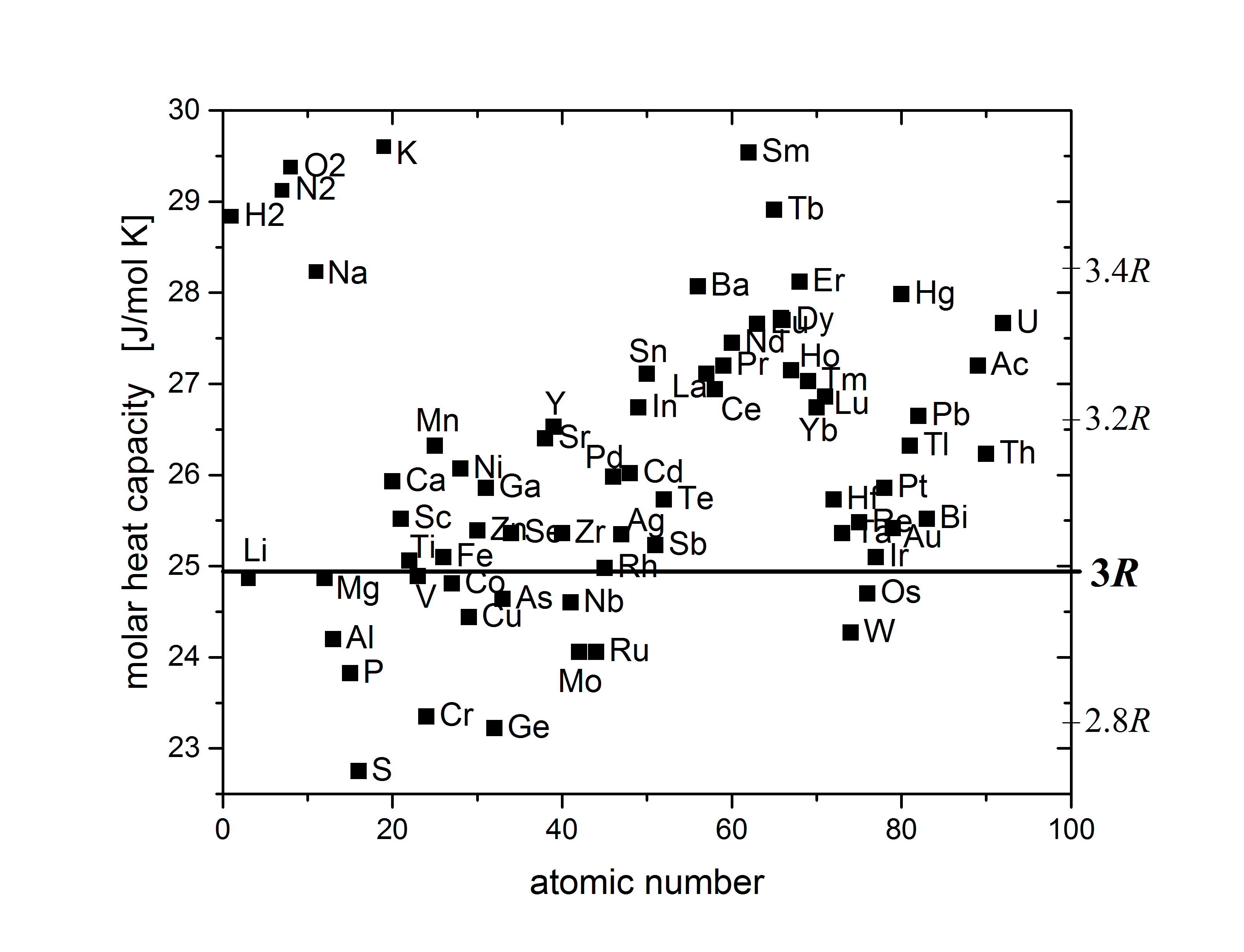 Molar heat capacity of most elements at 25 °C is in the range between 2.8 R and 3.4 R: Plot as a function of atomic number with a y range from 22.5 to 30 J/mol K. By Nick B. - Own work, CC BY-SA 4.0, Link
**File 1.2.15 ** GraphHeatCapacityElements_SelectedRange.png
### 1.3 Einstein Solids
**Definition 1.3.1 ** The **Einstein solid** is a quantum model of solids in the canonical ensemble that models the valence electrons of atoms as quantum harmonic oscillators with the following Hamiltonian $H$, where $\hat{p}$ is the momentum operator, $m$ is the mass, $k$ is the spring constant and $\hat{x}$ is the position operator.
\[\hat{H} = \frac{\hat{p}^2}{2m}+\frac{1}{2}k\hat{x}^2\]
**Result 1.3.2 ** The **eigenvalues of the 1D Harmonic oscillator** $E_n$ for the corresponding eigenstates $\ket{n}$ are given by the following equation for non-negative integer $n\in\mathbb{N}$.
\[E_n = \hbar\omega\left(n+\frac{1}{2}\right),\quad H\ket{n} = E_n\ket{n}, \quad \omega = \sqrt\frac{k}{m}\]
**Proposition 1.3.3 ** **Geometric series convergence** states that for $|r|<1$ the following infinite series converges to $1/(1-r)$.
\[\sum_{k=0}^\infty{r^k} = \frac{1}{1-r}\]
**Result 1.3.4 ** The **partition function of a 1D harmonic oscillator** $z_{1D}$ can be written as a geometric series:
\[z_{1D} = \sum_{n=0}^\infty{e^{-\beta E_n}} = \sum_{n=0}^\infty{e^{-\beta\hbar\omega(n+\frac{1}{2})}} = \frac{e^{\beta\hbar\omega/2}}{e^{\beta\hbar\omega}-1}\]
**Result 1.3.5 ** The **eigenvalues of the 3D Harmonic oscillator** $E_{n_x,n_y,n_z}$ for the corresponding eigenstates $\ket{n_x,n_y,n_z}$ are given by the following equation for non-negative integers $n_x,n_y,n_z\in\mathbb{N}$.
\[E_{n_x,n_y,n_z} = \hbar\omega\left(n_x+n_y+n_z+\frac{3}{2}\right)\]
\[H\ket{n_z,n_y,n_z} = E_{n_z,n_y,n_z}\ket{n}\]
\[\omega = \sqrt\frac{k}{m}\]
**Result 1.3.6 ** The **partition function of a 3D harmonic oscillator** $z_{3D}$ can be written in terms of the partition function for the 1D harmonic oscillator $z_{1D}$:
\[z_{3D} = \sum_{n_x,n_y,n_z=0}^\infty{e^{-\beta E_{n_x,n_y,n_z}}} = z_{1D}^3 = \left(\frac{e^{\beta\hbar\omega/2}}{e^{\beta\hbar\omega}-1}\right)^3\]
**Definition 1.3.7 ** The **Bose factor** is $n_B(\beta\hbar\omega) = \frac{1}{e^{\beta\hbar\omega}-1}$.
**Result 1.3.8 ** The **intensive energy of a Einstein solid** $u$ is the average energy per particle in a 3d solid determined by the following relation with temperature $T$.
\[u = -\frac{\partial}{\partial \beta}\log z_{3D} = -3\frac{\partial}{\partial \beta}\log z_{1D} \]
\[= 3\hbar\omega \left(n_B(\beta\hbar\omega)+\frac{1}{2} \right) = 3\hbar\omega \left( \frac{1}{e^{\beta\hbar\omega}-1} + \frac{1}{2} \right)\]
**Result 1.3.9 ** The **molar heat capacity of an Einstain solid** $c_{\text{mol}}$ satisfies the [Dulong Petit law](https://kaedon.net/l/5cdh) at high temperatures as $T\to\infty$ while converging to zero as $T\to0$.
\[c_{\text{mo}l} = \frac{C}{N_{mol}} = N_{Avogadro}\frac{\partial u}{\partial T} = 3R(\beta\hbar\omega)^2\frac{e^{\beta\hbar\omega}}{\left( e^{\beta\hbar\omega}-1 \right)^2}\]
**Definition 1.3.10 ** The **einstein temperature** denoted $T_E$ is the critical temperature where the molar heat capacity of an Einstein solid starts decreasing.
\[T_E = \frac{\hbar\omega}{k_B}\]
**Figure 1.3.11 Molar Heat Capacity of an Einstein Solid vs Temperature **
Molar heat capacity of most elements at 25 °C is in the range between 2.8 R and 3.4 R: Plot as a function of atomic number with a y range from 22.5 to 30 J/mol K. By Nick B. - Own work, CC BY-SA 4.0, Link
**File 1.2.15 ** GraphHeatCapacityElements_SelectedRange.png
### 1.3 Einstein Solids
**Definition 1.3.1 ** The **Einstein solid** is a quantum model of solids in the canonical ensemble that models the valence electrons of atoms as quantum harmonic oscillators with the following Hamiltonian $H$, where $\hat{p}$ is the momentum operator, $m$ is the mass, $k$ is the spring constant and $\hat{x}$ is the position operator.
\[\hat{H} = \frac{\hat{p}^2}{2m}+\frac{1}{2}k\hat{x}^2\]
**Result 1.3.2 ** The **eigenvalues of the 1D Harmonic oscillator** $E_n$ for the corresponding eigenstates $\ket{n}$ are given by the following equation for non-negative integer $n\in\mathbb{N}$.
\[E_n = \hbar\omega\left(n+\frac{1}{2}\right),\quad H\ket{n} = E_n\ket{n}, \quad \omega = \sqrt\frac{k}{m}\]
**Proposition 1.3.3 ** **Geometric series convergence** states that for $|r|<1$ the following infinite series converges to $1/(1-r)$.
\[\sum_{k=0}^\infty{r^k} = \frac{1}{1-r}\]
**Result 1.3.4 ** The **partition function of a 1D harmonic oscillator** $z_{1D}$ can be written as a geometric series:
\[z_{1D} = \sum_{n=0}^\infty{e^{-\beta E_n}} = \sum_{n=0}^\infty{e^{-\beta\hbar\omega(n+\frac{1}{2})}} = \frac{e^{\beta\hbar\omega/2}}{e^{\beta\hbar\omega}-1}\]
**Result 1.3.5 ** The **eigenvalues of the 3D Harmonic oscillator** $E_{n_x,n_y,n_z}$ for the corresponding eigenstates $\ket{n_x,n_y,n_z}$ are given by the following equation for non-negative integers $n_x,n_y,n_z\in\mathbb{N}$.
\[E_{n_x,n_y,n_z} = \hbar\omega\left(n_x+n_y+n_z+\frac{3}{2}\right)\]
\[H\ket{n_z,n_y,n_z} = E_{n_z,n_y,n_z}\ket{n}\]
\[\omega = \sqrt\frac{k}{m}\]
**Result 1.3.6 ** The **partition function of a 3D harmonic oscillator** $z_{3D}$ can be written in terms of the partition function for the 1D harmonic oscillator $z_{1D}$:
\[z_{3D} = \sum_{n_x,n_y,n_z=0}^\infty{e^{-\beta E_{n_x,n_y,n_z}}} = z_{1D}^3 = \left(\frac{e^{\beta\hbar\omega/2}}{e^{\beta\hbar\omega}-1}\right)^3\]
**Definition 1.3.7 ** The **Bose factor** is $n_B(\beta\hbar\omega) = \frac{1}{e^{\beta\hbar\omega}-1}$.
**Result 1.3.8 ** The **intensive energy of a Einstein solid** $u$ is the average energy per particle in a 3d solid determined by the following relation with temperature $T$.
\[u = -\frac{\partial}{\partial \beta}\log z_{3D} = -3\frac{\partial}{\partial \beta}\log z_{1D} \]
\[= 3\hbar\omega \left(n_B(\beta\hbar\omega)+\frac{1}{2} \right) = 3\hbar\omega \left( \frac{1}{e^{\beta\hbar\omega}-1} + \frac{1}{2} \right)\]
**Result 1.3.9 ** The **molar heat capacity of an Einstain solid** $c_{\text{mol}}$ satisfies the [Dulong Petit law](https://kaedon.net/l/5cdh) at high temperatures as $T\to\infty$ while converging to zero as $T\to0$.
\[c_{\text{mo}l} = \frac{C}{N_{mol}} = N_{Avogadro}\frac{\partial u}{\partial T} = 3R(\beta\hbar\omega)^2\frac{e^{\beta\hbar\omega}}{\left( e^{\beta\hbar\omega}-1 \right)^2}\]
**Definition 1.3.10 ** The **einstein temperature** denoted $T_E$ is the critical temperature where the molar heat capacity of an Einstein solid starts decreasing.
\[T_E = \frac{\hbar\omega}{k_B}\]
**Figure 1.3.11 Molar Heat Capacity of an Einstein Solid vs Temperature **
 Molar heat capacity predicted for an Einstein solid as a function of temperature. Public Domain, own work.
**File 1.3.11 ** MolarHeatCapacityofanEinstainSolidvsTemperature.svg
### 1.4 Debye Solids
Also see the Wikipedia article for this model: https://en.wikipedia.org/wiki/Debye_model
**Definition 1.4.1 ** The **Debye solid** is a model of solids in the canonical ensemble that models the collective phononic collective modes the atoms in the solid for some speed of sound $v$, the frequencies of the collect modes $\omega_k$ for wave number $\vec{k}$ are modeled by the following equations for the total energy $U$.
\[\omega_\vec{k} = v\abs{\vec{k}}\]
\[U = 3\sum_{\vec{k}}\hbar\omega_{\vec{k}}\left( n_B(\beta\hbar\omega_{\vec{k}}) + \frac{1}{2} \right) = 3\sum_{\vec{k}}\hbar\omega_{\vec{k}}\left( \frac{1}{e^{\beta\hbar\omega_{\vec{k}}}-1} + \frac{1}{2} \right)\]
**Definition 1.4.2 ** To calculate the modes of a Debye solid we assume **periodic boundary conditions** for some distance $L$ which is very large compared to the scale of the atom as to include all the lower frequency modes.
\[\vec{k}L = 2\pi\vec{n}\]
**Definition 1.4.3 ** The **Debye frequency** denoted $\omega_D$ is the maximum frequency of phonons in a Debye solid, defined in terms of the density $\rho$ and speed of sound $v$ of the solid.
\[\omega_D = \left(6\pi^2\rho\right)^{1/3}v\]
**Definition 1.4.4 ** The **Debye temperature** is $T_D = \frac{\hbar\omega_D}{k_B}$ where $\omega_D$ is the [debye frequency](https://kaedon.net/l/76mk).
**Definition 1.4.5 ** The **Debye density of states** denoted $g(\omega)$ of frequency modes $\omega$ with periodic boundary conditions $L$ and volume $V$ is the following function.
\[g(\omega) = \frac{L^3\omega^2}{2\pi^2V^3} = \frac{3N\omega^2}{\omega_D^3}\]
**Result 1.4.6 ** The sum of an isotropic function $f(\omega_{k})$ for all wave numbers $\vec{k}$ can be approximated as an integral of the density of states $g(\omega_{\vec{k}})$ and the function $f(\omega_{\vec{k}})$.
\[\sum_{\vec{k}}f(\omega_\vec{k})=\sum_\vec{k}f(v\abs{\vec{k}})=\sum_{\vec{n}\in\mathbb{N}^3}f\left(\frac{2\pi v}{L}\abs{\vec{n}}\right)\]
\[\approx\int d^3\vec{n} f\left(\frac{2\pi v}{L}\abs{\vec{n}}\right) = \left(\frac{L}{2\pi}\right)^3\int d^3\vec{k}f\left(v\abs{\vec{k}}\right)\]
\[= \frac{L^3}{2\pi^2}\int_0^{\omega_D} dk k^2 f(vk) = \frac{L^3}{2\pi^2 v^3}\int_0^{\omega_D} d\omega \omega^2 f(\omega) = \int_0^{\omega_D} d\omega g(\omega) f(\omega)\]
We set the maximum frequency of the integrate to $\omega_D$ because there are a finite number of atoms $N$. It turns out that there is a maximum frequency $\omega$ that these collective modes can exhibit. The next result proves that this cutoff frequency is indeed the [Debye frequency](https://kaedon.net/l/76mk) $\omega_D$.
**Result 1.4.8 ** The [Debye frequency](https://kaedon.net/l/^kjk0#76mk) is the maximum frequency in a Debye solid, because there are a finite number of atoms $N$ in a solid.
\[N = \sum_k 1 = \int_0^{\omega_D} d\omega g(\omega) = \int_0^{\omega_D} d\omega \frac{3N\omega^2}{\omega_D^3} = N\frac{\omega_D^3}{\omega_D^3} = N\]
**Result 1.4.9 ** The **total energy** $U$ **of a Debye solid** is given by the following integral of the [Debye density of states](https://kaedon.net/l/^kjk0#7n9k) $g(\omega)$ and the [Bose factor](https://kaedon.net/l/^kjk0#c06t) $n_B(\beta\hbar\omega)$.
\[U = \int_0^{\omega_D} d\omega g(\omega) 3\hbar\omega\left( n_B(\beta\hbar\omega) + \frac{1}{2} \right) = \int_0^{\omega_D} d\omega \frac{3N\omega^2}{\omega_D^3} 3\hbar\omega\left( \frac{1}{e^{\beta\hbar\omega}-1} + \frac{1}{2} \right)\]
**Result 1.4.10 ** The **molar heat capacity** $c_{mol}$ **of a Debye solid** is given by the following integral.
\[c_{mol} = \frac{1}{N_{mol}}\frac{\partial U}{\partial T} = \frac{1}{N_{mol}}\frac{\partial}{\partial T}\int_0^{\omega_D} d\omega g(\omega) 3\hbar\omega\left( n_B(\beta\hbar\omega) + \frac{1}{2} \right) \]
\[= \frac{1}{N_{mol}}\frac{\partial}{\partial T}\int_0^{\omega_D} d\omega \frac{3N\omega^2}{\omega_D^3} 3\hbar\omega\left( \frac{1}{e^{\beta\hbar\omega}-1} + \frac{1}{2} \right)\]
\[=3k_BN_{Avogadro}\frac{(\beta\hbar\omega_D)^2e^{\beta\hbar\omega} }{(e^{\beta\hbar\omega}-1)^2} =3R\frac{(\beta\hbar\omega_D)^2e^{\beta\hbar\omega} }{(e^{\beta\hbar\omega}-1)^2}\]
**Figure 1.4.11 Debye vs. Einstein **
Molar heat capacity predicted for an Einstein solid as a function of temperature. Public Domain, own work.
**File 1.3.11 ** MolarHeatCapacityofanEinstainSolidvsTemperature.svg
### 1.4 Debye Solids
Also see the Wikipedia article for this model: https://en.wikipedia.org/wiki/Debye_model
**Definition 1.4.1 ** The **Debye solid** is a model of solids in the canonical ensemble that models the collective phononic collective modes the atoms in the solid for some speed of sound $v$, the frequencies of the collect modes $\omega_k$ for wave number $\vec{k}$ are modeled by the following equations for the total energy $U$.
\[\omega_\vec{k} = v\abs{\vec{k}}\]
\[U = 3\sum_{\vec{k}}\hbar\omega_{\vec{k}}\left( n_B(\beta\hbar\omega_{\vec{k}}) + \frac{1}{2} \right) = 3\sum_{\vec{k}}\hbar\omega_{\vec{k}}\left( \frac{1}{e^{\beta\hbar\omega_{\vec{k}}}-1} + \frac{1}{2} \right)\]
**Definition 1.4.2 ** To calculate the modes of a Debye solid we assume **periodic boundary conditions** for some distance $L$ which is very large compared to the scale of the atom as to include all the lower frequency modes.
\[\vec{k}L = 2\pi\vec{n}\]
**Definition 1.4.3 ** The **Debye frequency** denoted $\omega_D$ is the maximum frequency of phonons in a Debye solid, defined in terms of the density $\rho$ and speed of sound $v$ of the solid.
\[\omega_D = \left(6\pi^2\rho\right)^{1/3}v\]
**Definition 1.4.4 ** The **Debye temperature** is $T_D = \frac{\hbar\omega_D}{k_B}$ where $\omega_D$ is the [debye frequency](https://kaedon.net/l/76mk).
**Definition 1.4.5 ** The **Debye density of states** denoted $g(\omega)$ of frequency modes $\omega$ with periodic boundary conditions $L$ and volume $V$ is the following function.
\[g(\omega) = \frac{L^3\omega^2}{2\pi^2V^3} = \frac{3N\omega^2}{\omega_D^3}\]
**Result 1.4.6 ** The sum of an isotropic function $f(\omega_{k})$ for all wave numbers $\vec{k}$ can be approximated as an integral of the density of states $g(\omega_{\vec{k}})$ and the function $f(\omega_{\vec{k}})$.
\[\sum_{\vec{k}}f(\omega_\vec{k})=\sum_\vec{k}f(v\abs{\vec{k}})=\sum_{\vec{n}\in\mathbb{N}^3}f\left(\frac{2\pi v}{L}\abs{\vec{n}}\right)\]
\[\approx\int d^3\vec{n} f\left(\frac{2\pi v}{L}\abs{\vec{n}}\right) = \left(\frac{L}{2\pi}\right)^3\int d^3\vec{k}f\left(v\abs{\vec{k}}\right)\]
\[= \frac{L^3}{2\pi^2}\int_0^{\omega_D} dk k^2 f(vk) = \frac{L^3}{2\pi^2 v^3}\int_0^{\omega_D} d\omega \omega^2 f(\omega) = \int_0^{\omega_D} d\omega g(\omega) f(\omega)\]
We set the maximum frequency of the integrate to $\omega_D$ because there are a finite number of atoms $N$. It turns out that there is a maximum frequency $\omega$ that these collective modes can exhibit. The next result proves that this cutoff frequency is indeed the [Debye frequency](https://kaedon.net/l/76mk) $\omega_D$.
**Result 1.4.8 ** The [Debye frequency](https://kaedon.net/l/^kjk0#76mk) is the maximum frequency in a Debye solid, because there are a finite number of atoms $N$ in a solid.
\[N = \sum_k 1 = \int_0^{\omega_D} d\omega g(\omega) = \int_0^{\omega_D} d\omega \frac{3N\omega^2}{\omega_D^3} = N\frac{\omega_D^3}{\omega_D^3} = N\]
**Result 1.4.9 ** The **total energy** $U$ **of a Debye solid** is given by the following integral of the [Debye density of states](https://kaedon.net/l/^kjk0#7n9k) $g(\omega)$ and the [Bose factor](https://kaedon.net/l/^kjk0#c06t) $n_B(\beta\hbar\omega)$.
\[U = \int_0^{\omega_D} d\omega g(\omega) 3\hbar\omega\left( n_B(\beta\hbar\omega) + \frac{1}{2} \right) = \int_0^{\omega_D} d\omega \frac{3N\omega^2}{\omega_D^3} 3\hbar\omega\left( \frac{1}{e^{\beta\hbar\omega}-1} + \frac{1}{2} \right)\]
**Result 1.4.10 ** The **molar heat capacity** $c_{mol}$ **of a Debye solid** is given by the following integral.
\[c_{mol} = \frac{1}{N_{mol}}\frac{\partial U}{\partial T} = \frac{1}{N_{mol}}\frac{\partial}{\partial T}\int_0^{\omega_D} d\omega g(\omega) 3\hbar\omega\left( n_B(\beta\hbar\omega) + \frac{1}{2} \right) \]
\[= \frac{1}{N_{mol}}\frac{\partial}{\partial T}\int_0^{\omega_D} d\omega \frac{3N\omega^2}{\omega_D^3} 3\hbar\omega\left( \frac{1}{e^{\beta\hbar\omega}-1} + \frac{1}{2} \right)\]
\[=3k_BN_{Avogadro}\frac{(\beta\hbar\omega_D)^2e^{\beta\hbar\omega} }{(e^{\beta\hbar\omega}-1)^2} =3R\frac{(\beta\hbar\omega_D)^2e^{\beta\hbar\omega} }{(e^{\beta\hbar\omega}-1)^2}\]
**Figure 1.4.11 Debye vs. Einstein **
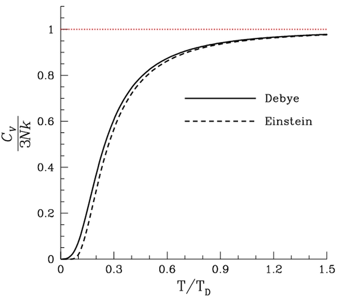 Predicted heat capacity as a function of temperature. Public Domain, Link
**File 1.4.11 ** DebyeVSEinstein.jpg
## 2 Drude-Lorentz Theory
### 2.1 Drude Model
**Definition 2.1.1 ** The **Drude model** is a simple model of electron motion and scattering in a material with a differential equation describing of the momentum $\vec{p}$ of electrons experiencing the Lorentz force from an external electric field $\vec{E}$, magnetic field $\vec{B}$ and scattering with a mean scattering time of $\tau$.
\[\frac{\partial \vec{p}}{\partial t} = -e\left( \vec{E} + \frac{1}{m}\vec{p}\times\vec{B} \right) + \frac{\vec{p}}{\tau}\]
Despite the apparent simplicity of the [Drude Model](https://kaedon.net/l/73pc), it has been wildly successful at predicting a variety of phenomena related to electron transport in solids. Some of these phenomena include:
- [Ohm's Law](https://kaedon.net/l/d4em)
- [The Hall Effect](https://kaedon.net/l/pt5f)
The following sections will describe each of these phenomena using the [Drude Model](https://kaedon.net/l/73pc). The drude model can then also be expanded into a complete thermodynamic theory for electrons with the [Drude-Lorentz gas](https://kaedon.net/l/tf4d). Which allows it to at least conceptually explain the following phenomena:
- [Weidermann's Franz Law](https://kaedon.net/l/tf4d)
- [Transparency of Materials](https://kaedon.net/l/^kjk0#6kn0)
### 2.2 Ohm's Law
**Definition 2.2.1 ** A **current density** denoted $\vec{j}$ is a vector field describing the average density of charge flowing through a particular point in space per second.
**Definition 2.2.2 ** The **electric conductivity** denoted $\sigma$ of a material is the coefficient or tensor that relates the electric field $\vec{E}$ to the current density $\vec{j}$.
\[\vec{j} = \sigma \vec{E}\]
**Definition 2.2.3 ** The **resistivity** denoted $\rho$ of a material is the coefficient or tensor that relates the current density $\vec{\rho}$ flowing through a material with the electric field $\vec{E}$ required to drive that current.
\[\vec{E} = \rho\vec{j}\]
**Corollary 2.2.4 ** The [conductivity](https://kaedon.net/l/1htz) $\sigma$ and [resistivity](https://kaedon.net/l/h144) $\rho$ of a material are inverses of each other.
\[\sigma = \frac{1}{\rho},\quad \rho = \frac{1}{\sigma}\]
**Definition 2.2.5 ** The **Drude conducitivity** denoted $\sigma_D$ is the [electric conductivity](https://kaedon.net/l/1htz) predicted by the Drude model for a pure electric field $\vec{E}$ ($\vec{B}=\vec{0}$) where $\tau$ is the mean scattering time, $n_e$ is number of electrons, $e$ is the elemental charge and $m_e$ is the mass of charge carriers.
\[\vec{j}_D = \frac{e^2n_e\tau}{m_e}\vec{E} = \sigma_D\vec{E}\]
**Definition 2.2.6 ** The **resistance** denoted $R$ of a prism of material with cross sectional area $A$, length $L$ and resistivity $\rho$ is given by the following relation.
\[R = \rho \frac{\ell}{A}\]
Predicted heat capacity as a function of temperature. Public Domain, Link
**File 1.4.11 ** DebyeVSEinstein.jpg
## 2 Drude-Lorentz Theory
### 2.1 Drude Model
**Definition 2.1.1 ** The **Drude model** is a simple model of electron motion and scattering in a material with a differential equation describing of the momentum $\vec{p}$ of electrons experiencing the Lorentz force from an external electric field $\vec{E}$, magnetic field $\vec{B}$ and scattering with a mean scattering time of $\tau$.
\[\frac{\partial \vec{p}}{\partial t} = -e\left( \vec{E} + \frac{1}{m}\vec{p}\times\vec{B} \right) + \frac{\vec{p}}{\tau}\]
Despite the apparent simplicity of the [Drude Model](https://kaedon.net/l/73pc), it has been wildly successful at predicting a variety of phenomena related to electron transport in solids. Some of these phenomena include:
- [Ohm's Law](https://kaedon.net/l/d4em)
- [The Hall Effect](https://kaedon.net/l/pt5f)
The following sections will describe each of these phenomena using the [Drude Model](https://kaedon.net/l/73pc). The drude model can then also be expanded into a complete thermodynamic theory for electrons with the [Drude-Lorentz gas](https://kaedon.net/l/tf4d). Which allows it to at least conceptually explain the following phenomena:
- [Weidermann's Franz Law](https://kaedon.net/l/tf4d)
- [Transparency of Materials](https://kaedon.net/l/^kjk0#6kn0)
### 2.2 Ohm's Law
**Definition 2.2.1 ** A **current density** denoted $\vec{j}$ is a vector field describing the average density of charge flowing through a particular point in space per second.
**Definition 2.2.2 ** The **electric conductivity** denoted $\sigma$ of a material is the coefficient or tensor that relates the electric field $\vec{E}$ to the current density $\vec{j}$.
\[\vec{j} = \sigma \vec{E}\]
**Definition 2.2.3 ** The **resistivity** denoted $\rho$ of a material is the coefficient or tensor that relates the current density $\vec{\rho}$ flowing through a material with the electric field $\vec{E}$ required to drive that current.
\[\vec{E} = \rho\vec{j}\]
**Corollary 2.2.4 ** The [conductivity](https://kaedon.net/l/1htz) $\sigma$ and [resistivity](https://kaedon.net/l/h144) $\rho$ of a material are inverses of each other.
\[\sigma = \frac{1}{\rho},\quad \rho = \frac{1}{\sigma}\]
**Definition 2.2.5 ** The **Drude conducitivity** denoted $\sigma_D$ is the [electric conductivity](https://kaedon.net/l/1htz) predicted by the Drude model for a pure electric field $\vec{E}$ ($\vec{B}=\vec{0}$) where $\tau$ is the mean scattering time, $n_e$ is number of electrons, $e$ is the elemental charge and $m_e$ is the mass of charge carriers.
\[\vec{j}_D = \frac{e^2n_e\tau}{m_e}\vec{E} = \sigma_D\vec{E}\]
**Definition 2.2.6 ** The **resistance** denoted $R$ of a prism of material with cross sectional area $A$, length $L$ and resistivity $\rho$ is given by the following relation.
\[R = \rho \frac{\ell}{A}\]
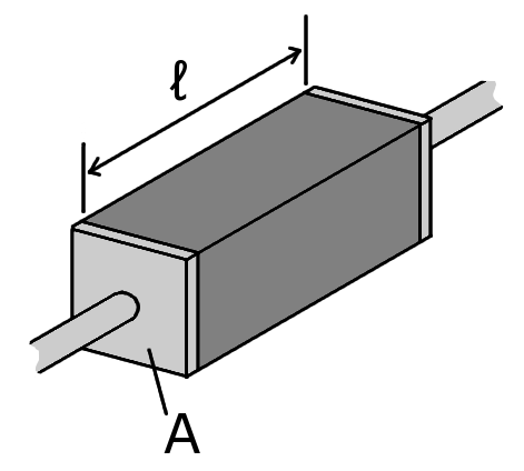 **File 2.2.6 ** Resistance_geometry.png
**Law 2.2.7 ** **Ohm's law** states that the total current $I$ flowing through a material is equal to the resistance $R$ times the bias voltage across the material $V$.
\[V = IR\]
### 2.3 The Hall Effect
**Definition 2.3.1 ** The **cyclotron frequency** denoted $\omega_c$ is the frequency at which an electron would spin in a magnetic field of strength $B$, with elemental charge $e$ and electron mass $m_e$.
\[\omega_c = \frac{eB}{m_e}\]
**Definition 2.3.2 ** The **hall effect** is the production of an electric field $\vec{E}_{\text{hall}}$ (called the **hall field**) across a material in the direction of the cross product between the external electric field $\vec{E}_{\text{ext}}$ and the magnetic field $\vec{B}$.
**Result 2.3.3 ** The **classical hall effect** is the hall effect as predicted by solving the equilibrium condition $\frac{\partial \vec{p}}{\partial t} = 0$ for the [Drude Model](https://kaedon.net/l/73pc) in 2 dimensions with a magnetic field $\vec{B}=B\hat{z}$ perpendicular to the plane and an in-plane electric field $\vec{E} = E_x\hat{x} + E_y\hat{y}$.
\[0=-eE_x - \omega_c p_y - \frac{p_x}{\tau}, \quad 0=-eE_y + \omega_c p_x - \frac{p_y}{\tau}\]
\[\vec{p} = \frac{-e\tau}{1+(\omega_c\tau)^2}\begin{pmatrix}1 & -\omega_c\tau\\ \omega_c\tau & 1\end{pmatrix}\vec{E}\]
**Figure 2.3.4 Hall Effect Diagram **
**File 2.2.6 ** Resistance_geometry.png
**Law 2.2.7 ** **Ohm's law** states that the total current $I$ flowing through a material is equal to the resistance $R$ times the bias voltage across the material $V$.
\[V = IR\]
### 2.3 The Hall Effect
**Definition 2.3.1 ** The **cyclotron frequency** denoted $\omega_c$ is the frequency at which an electron would spin in a magnetic field of strength $B$, with elemental charge $e$ and electron mass $m_e$.
\[\omega_c = \frac{eB}{m_e}\]
**Definition 2.3.2 ** The **hall effect** is the production of an electric field $\vec{E}_{\text{hall}}$ (called the **hall field**) across a material in the direction of the cross product between the external electric field $\vec{E}_{\text{ext}}$ and the magnetic field $\vec{B}$.
**Result 2.3.3 ** The **classical hall effect** is the hall effect as predicted by solving the equilibrium condition $\frac{\partial \vec{p}}{\partial t} = 0$ for the [Drude Model](https://kaedon.net/l/73pc) in 2 dimensions with a magnetic field $\vec{B}=B\hat{z}$ perpendicular to the plane and an in-plane electric field $\vec{E} = E_x\hat{x} + E_y\hat{y}$.
\[0=-eE_x - \omega_c p_y - \frac{p_x}{\tau}, \quad 0=-eE_y + \omega_c p_x - \frac{p_y}{\tau}\]
\[\vec{p} = \frac{-e\tau}{1+(\omega_c\tau)^2}\begin{pmatrix}1 & -\omega_c\tau\\ \omega_c\tau & 1\end{pmatrix}\vec{E}\]
**Figure 2.3.4 Hall Effect Diagram **
 Hall Effect Measurement Setup for Electrons. An external field $E_x$ is applied in the x direction and a magnetic field $B_z$ is applied in the z direction, resulting in a hall field $E_y$ in the y direction. Public Domain, Link
**File 2.3.4 ** Hall_Effect_Measurement_Setup_for_Electrons.svg
**Result 2.3.5 ** The **classical hall field** $\vec{E}_{\text{hall}}$ for external electric field $\vec{E}_{\text{ext}}$ and magnetic field $\vec{B}$ can be written in terms of the [cyclotron frequency](https://kaedon.net/l/k3cc) $\omega_c$ and [mean scattering time](https://kaedon.net/l/73pc) $\tau$
\[\vec{E}_{\text{hall}} = \omega_c\tau(\vec{B}\times\vec{E}_{\text{ext}})\]
**Definition 2.3.6 ** The **hall coefficient** denoted $R_H$ is the measurable ratio between the hall field $E_y$ and the product of the current $J_x$ and $B_z$ applied to drive that hall field. The Drude model predicts that this quantity is related to the charge carrier density $n_e$.
\[R_H = \frac{E_y}{J_xB_z} = \frac{-\omega_c\tau E_x}{J_x B_z} = \frac{-1}{en_e}\]
### 2.4 Weiderman Franz Law
**Definition 2.4.1 ** The **temperature gradient** denoted $\vec{\nabla} T(\vec{r})$ is the the gradient of temperature $T(\vec{r})$ at position $\vec{r}$ in a material.
**Definition 2.4.2 ** The **heat current** denoted $\vec{j}_q$ is the rate of energy transfer through a material due to temperature gradient.
**Definition 2.4.3 ** The **thermal conductivity** denoted $\kappa$ of a material is the coefficient that relates the temperature gradient $\vec\nabla T$ to the heat current $\vec{j}_q$.
\[\vec{j}_q = -\kappa\vec\nabla T\]
**Definition 2.4.4 ** The **Drude thermal conductivity** denoted $\kappa_D$ is the thermal conductivity predicted by the predicted by the Drude model with density of electron $n$, average thermal velocity $v = \frac{k_B T}{m_e}$, mean scattering time $\tau$ and molar heat capacity $c_{\text{el,mol}} = \frac{\partial u}{\partial T}$
\[\kappa_D = nv^2\tau\frac{\partial u}{\partial T} = n \frac{k_BT}{m_e}\tau c_{\text{el,mol}}\]
**Definition 2.4.5 ** The **Lorentz number** denoted $L$ is the proportionality constant that relates the thermal conductivity $\kappa$ to the electric conductivity $\sigma$ at temperature $T$.
\[L = \frac{\kappa}{\sigma T}\]
**Result 2.4.6 ** The **Drude Weiderman Franz Law** describes the [Lorentz Number](https://kaedon.net/l/217r) predicted by the Drude model.
\[L = \frac{\kappa}{\sigma T} = \frac{n \frac{k_BT}{m_e}\tau c_{\text{el,mol}}}{\frac{e^2n_e\tau}{m_e} T} = \frac{k_B c_{\text{el,mol}}}{e^2} = \frac{3}{2}\left(\frac{k_B}{e}\right)^2\]
### 2.5 Drude-Lorentz Gas
**Definition 2.5.1 ** The **distribution function** denoted $f(\vec{r},\vec{p})$ for classical systems is the density of particle in position-momentum phase space. For $N$ particles at positions $\vec{r}_n$ and momenta $\vec{p}_n$, is given by the following sum of 3D Dirac deltas $\delta^3$.
\[f(\vec{r},\vec{p}) = \sum_{n=1}^N\delta^3(\vec{r}-\vec{r}_n)\delta^3(\vec{p}-\vec{p}_n)\]
**Definition 2.5.2 ** A **generic physical observable** $A$ **of distribution function** $f(\vec{r},\vec{p})$ is given the following integral where $A(\vec{r},\vec{p})$ is the contribution to that observable by a single particle in the distribution function.
\[A = \int d^3\vec{r}d^3\vec{p} f(\vec{r},\vec{p})A(\vec{r},\vec(p))\]
**Result 2.5.3 ** The **particle number** $N$ **of a distribution function** $f(\vec{r},\vec{p})$ is given by $N = \int d^3\vec{r}d^3\vec{p} f(\vec{r},\vec{p})$.
**Result 2.5.4 ** The **particle density** $n(\vec{r})$ **of a distribution function** $f(\vec{r},\vec{p})$ is given by $n(\vec{r}) = \int d^3\vec{p} f(\vec{r},\vec{p})$.
**Result 2.5.5 ** The **current density** $\vec{j}(\vec{r})$ **of a distribution function** $f(\vec{r},\vec{p})$ is given by $\vec{j}(\vec{r}) = \int d^3\vec{p} f(\vec{r},\vec{p}) \left(\frac{-e\vec{p}}{m}\right)$.
**Result 2.5.6 ** The **total energy** $U$ **of a distribution function** $f(\vec{r},\vec{p})$ is given by $U = \int d^3\vec{r}d^3\vec{p} f(\vec{r},\vec{p})$.
**Result 2.5.7 ** The **total energy** $\vec{p}$ **of a distribution function** $f(\vec{r},\vec{p})$ is given by $\vec{p} = \int d^3\vec{r}d^3\vec{p} f(\vec{r},\vec{p}) \vec{p}$.
**Definition 2.5.8 ** A **Drude-Lorentz gas** is a classical model of electrons in a solid that assume electrons relax to a Maxwell-Boltzmann equilibrium via simple random scattering with mean lifetime $\tau$. See the [supplementary note](https://kaedon.nethttps://kaedon.net/l/t4zf) for a guided derivation. The model describes the behavior of a distribution $f(\vec{r},\vec{p})$ of electrons with the following differential equation such that the equilibrium condition is the Maxwell-Boltzmann distribution $f_0(\vec{r},\vec{p})$.
\[\frac{d}{dt}f(\vec{r},\vec{p}) = \frac{f_0(\vec{r},\vec{p})-f(\vec{r},\vec{p})}{\tau}-\frac{\partial \vec{r}}{\partial t}\cdot\nabla_{\vec{r}}f(\vec{r},\vec{p}) - \frac{\partial \vec{p}}{\partial t}\cdot\nabla_{\vec{p}}f(\vec{r},\vec{p})\]
\[f_0(\vec{r},\vec{p}) = \frac{n e^{-\beta p^2/(2m)}}{(2\pi m_e k_B T)^{3/2}}\]
**Result 2.5.9 ** For weak fields $\vec{E}$ and $\vec\nabla T$, the distribution of the Drude-Lortenz Gas can be approximated by the following.
\[f(\vec{r},\vec{p}) \approx f_0 + \frac{\partial f}{\partial E}\vec{E} + \frac{\partial f}{\partial \vec\nabla T} \vec{\nabla}T\]
**Definition 2.5.10 ** The **linear response operators** denoted $L_{\alpha\beta}$ for $\alpha,\beta\in\{1,2\}$ describe the linear relationship for small electric fields $\vec{E}$ and temperature gradients $\vec\nabla T$ with the current $\vec{j}$ and heat current $\vec{j}_q$.
\[\begin{pmatrix} \vec{j}\\ \vec{j}_q \end{pmatrix} = \begin{pmatrix} L_{11} & L_{12} \\ L_{21} & L_{22} \end{pmatrix}\begin{pmatrix} \vec{E} \\ -\vec{\nabla}T\end{pmatrix}\]
**Result 2.5.11 ** The **Drude-Lorentz electric conductivity** is the electric conductivity $\sigma$ predicted by the Drude-Lorentz model for small electric fields $\vec{E}$ and $\vec\nabla T =0$,
\[\vec{j} = \sigma \vec{E} = L_{11} \vec{E} = \frac{ne\tau}{m_e}\vec{E}\]
**Result 2.5.12 ** The **Drude-Lorentz heat conductivity** is the heat conductivity $\kappa$ predicted bt the Drude-Lorentz model for small temperature gradients $\vec\nabla T$ and $\vec{E} = 0$,
\[\vec{j}_q = -\kappa \vec\nabla T = -\left(L_{22} - \frac{L_{12}L_{21}}{L_{22}}\right)\vec\nabla T = -\frac{5}{2}\frac{k_B^2 nT\tau}{m_e}\vec\nabla T\]
**Result 2.5.13 ** The **Drude-Lorentz seebeck coefficient** is the seebeck coefficient $S$ predicted by the Drude-Lorentz model for small temperature gradients $\vec\nabla T$ and $\vec{j} = 0$,
\[\vec{E} = S\vec\nabla T = \frac{L_{12}}{L_{11}}\vec\nabla T = -\frac{k_B}{e} \vec\nabla T\]
**Result 2.5.14 ** The **Drude-Lorentz peltiercoefficient** is the peltier coefficient $\Pi$ predicted by the Drude-Lorentz model for small currents $\vec{j}\neq 0$ and $\vec\nabla T = 0$,
\[\vec{j}_q = \Pi \vec{j} = ST\vec{j} = \frac{k_BT}{e}\vec{j}\]
**Result 2.5.15 ** The **Drude-Lorentz molar heat capacity** is the molar heat capacity $c_{\text{el,mol}}$ predicted by the Drude-Lorentz model,
\[c_{\text{el,mol}} = \frac{3}{2} R Z\]
**Law 2.5.16 ** The **Drude-Lorentz Wiedemann–Franz law** describes the [Lorentz Number](https://kaedon.net/l/217r) predicted by the Drude-Lorentz model.
\[L = \frac{\kappa}{\sigma L} = \frac{5}{2}\left( \frac{k_B}{e} \right)^2\]
**Note 2.5.17 ** While the Drude-Lorentz gas successfully predicts the existence of these effects, they value of the coefficients are off by orders of magnitude.
### 2.6 Transparency
**Definition 2.6.1 ** A **plane wave** with frequency $\omega$ is an electric field $\vec{E}(\vec{r},t)$ of the following form.
\[\vec{E}(\vec{r},t) = \vec{E}_0\cos(\vec{k}\cdot\vec{r} - \omega t)\]
**Definition 2.6.2 ** The **Drude plasma frequency** denoted $\omega_p$ is the plasma frequency of a Drude metal.
**Result 2.6.3 ** For $\omega\tau >> 1$
\[\omega_p = \sqrt\frac{\sigma_0}{\varepsilon_0 \tau} = \sqrt{\frac{ne^2}{m_e\varepsilon_0}}\]
**Result 2.6.4 ** Penetration depth
**Result 2.6.5 ** wavelengths at high frequency
**Result 2.6.6 ** plasma wavelength
## 3 Sommerfeld Theory
### 3.1 One Electron
**Definition 3.1.1 ** The **single electron Hamiltonian** is the quantum mechanical Hamiltonian consisting on a single electron.
\[H = \frac{p^2}{2m},\quad \vec{p} = -i\hbar\vec\nabla_r\]
**Result 3.1.2 ** The **energy eigenstates of a single electron** with volume $V=L^3$ are given by the following equation for positive integers $n_x,n_y,n_z\in\mathbb{N}$ and spins $\sigma \in \{1,-1\}$,
\[\phi_{\vec{k},\sigma}(\vec{r}) = \frac{1}{\sqrt{V}}e^{i\vec{k}\cdot\vec{r}}\]
\[E(\vec{k},\sigma) = \frac{\hbar^2 k^2}{2m},\quad \vec{k} = \frac{2\pi}{L}\vec{n}\]
### 3.2 Two Electrons
**Definition 3.2.1 ** The **two electron Hamiltonian** is the quantum mechanical Hamiltonian consisting of two electrons with spin.
\[H = \sum_{n=1,2}\frac{p_n^2}{2m},\quad \vec{p}_n = -i\hbar\vec\nabla_r\]
The two electron system must also have exchange symmetry, that is energy states are indistinguishable under particle exchange.
**Definition 3.2.2 ** The **exchange operator** denoted $\hat{P}$ is the operator that swaps the particles of a state.
\[\hat{P}_{1,2}\Psi(\vec{r}_1,\sigma_1,\vec{r}_2,\sigma_2) = \Psi(\vec{r}_2,\sigma_2,\vec{r}_1,\sigma_1)\]
**Definition 3.2.3 ** A system has **exchange symmetry** iff its states are unaffected by even particle exchanges, that is
\[\hat{P}^2\Psi = \Psi\]
**Definition 3.2.4 ** A **boson** is a particle with exchange symmetry whose bare states are unaffected by particle exchange,
\[\hat{P}\Psi = \Psi\]
**Definition 3.2.5 ** A **fermion** is a particle with exchange symmetry whose bare states are negated by particle exchange,
\[\hat{P}\Psi = -\Psi\]
**Result 3.2.6 ** The **energy eigenstates of two electrons** with exchange symmetry, volume $V=L^3$ are given by the following equation for positive integers $\vec{n}_1,\vec{n_2}\in\mathbb{N}^3$ and spins $\sigma_1,\sigma_2 \in \{1,-1\}$,
\[\Psi(\vec{r}_1,\sigma,\vec{r}_2,\sigma_2) = \bra{\vec{r}_1,\sigma,\vec{r}_2,\sigma_2}\ket{\Psi} = \frac{1}{\sqrt{2}}\text{det}\left[\bra{\vec{r}_n,\sigma_n}\ket{\vec{k}_m,\tau_m}\right]_{n,m\in\{1,2\}}\]
\[\bra{\vec{r}_n,\sigma_n}\ket{\vec{k}_m,\tau_m} = \delta_{\sigma_n,\tau_m}\frac{1}{\sqrt{V}}e^{i\vec{k}_m\cdot\vec{r}_n}\]
\[E(\vec{k}_1,\sigma_1,\vec{k}_2,\sigma_2) = \frac{\hbar^2}{2m}\left(k_1^2 + k_2^2\right),\quad \vec{k} = \frac{2\pi}{L}\vec{n}\]
The two electrons cannot occupy the same state.
### 3.3 Sommerfeld Gas
**Definition 3.3.1 ** The **many electron Hamiltonian** is the quantum mechanical Hamiltonian consisting of $N$ electrons with spin.
\[H = \sum_{n=1}^N\frac{p_n^2}{2m},\quad \vec{p}_n = -i\hbar\vec\nabla_r\]
The electron system must also have exchange symmetry, that is energy states are indistinguishable under particle exchange.
**Result 3.3.2 ** The **energy eigenstates of many electrons** with exchange symmetry, volume $V=L^3$ are given by the following equation for positive integers $\vec{n}_1,\dots,\vec{n_N}\in\mathbb{N}^3$ and spins $\sigma_1,\dots,\sigma_N \in \{1,-1\}$,
\[\Psi(\vec{r}_1,\sigma,\dots,\vec{r}_N,\sigma_N) = \bra{\vec{r}_1,\sigma,\dots,\vec{r}_N,\sigma_N}\ket{\Psi} = \frac{1}{\sqrt{2}}\text{det}\left[\bra{\vec{r}_n,\sigma_n}\ket{\vec{k}_m,\tau_m}\right]_{n,m\in\{1,\dots,N\}}\]
\[\bra{\vec{r}_n,\sigma_n}\ket{\vec{k}_m,\tau_m} = \delta_{\sigma_n,\tau_m}\frac{1}{\sqrt{V}}e^{i\vec{k}_m\cdot\vec{r}_n}\]
\[E(\vec{k}_1,\sigma_1,\dots,\vec{k}_N,\sigma_N) = \frac{\hbar^2}{2m}\sum_{n=1}^Nk_n^2,\quad \vec{k}_n = \frac{2\pi}{L}\vec{n}_n\]
The eigenstates are antisymmetric (have exchange symmetry) for any two electron exchange. A state is an eigenstates iff $(\vec{k}_n,\tau_n)\neq(\vec{k}_m,\tau_m)$ $\forall n\neq m$.
**Result 3.3.3 ** The **energy of many identical electrons** $E$ can be written as a sum of occupied states,
\[E = \sum_{\vec{k},\sigma} \varepsilon_{\vec{k},\sigma} n_{\vec{k},\sigma} = \sum_{\vec{k},\sigma} \frac{\hbar k^2}{2m} n_{\vec{k},\sigma}\]
\[n_{\vec{k},\sigma} \in \{0,1\},\quad N = \sum_{\vec{k},\sigma} n_{\vec{k},\sigma}\]
**Definition 3.3.4 ** The **Sommerfeld gas** is a system of many identical electrons in the grand canonical ensemble at temperature $T=1/k_B\beta$, volume $V$ and chemical potential $\mu$ with the following grand partition function,
\[\mathscr{z} = \sum_{\{n_{\vec{k},\sigma}\}} e^{-\beta(E-\mu N)} = \sum_{\{n_{\vec{k},\sigma}\}} e^{-\beta\sum_{\vec{k},\sigma}n_{\vec{k},\sigma}(\varepsilon_{\vec{k},\sigma}-\mu)} = \prod_{\vec{k},\sigma} \left( 1 + e^{-\beta\left(\varepsilon_{\vec{k},\sigma}-\mu\right)} \right)\]
**Definition 3.3.5 ** The **Fermi Dirac distribution** is $f_{FD}(x) = \frac{1}{1+e^x}$
**Result 3.3.6 ** The **electron number of a Sommerfeld gas** can be written in terms of the Fermi Dirac distribution.
\[N = k_B T\frac{\partial \log\mathcal{z}}{\partial \mu} = \sum_{\vec{k},\sigma} f_{\vec{k},\sigma} = \sum_{\vec{k},\sigma} f_{FD}(\beta(\varepsilon_{\vec{k},\sigma} - \mu)) = 2 \frac{V}{(2\pi)^3}\int d^3\vec{k} f_{FD}(\beta(\varepsilon_{\vec{k},\sigma} - \mu))\]
**Result 3.3.7 ** The **total energy of a Sommerfeld gas** can be written in terms of the Fermi Dirac distribution.
\[U = -\frac{\partial \log\mathcal{z}}{\partial \beta} + \mu N = \sum_{\vec{k},\sigma}f_{\vec{k},\sigma} \varepsilon_{\vec{k},\sigma}= 2 \frac{V}{(2\pi)^3}\int d^3\vec{k} f_{FD}(\beta(\varepsilon_{\vec{k},\sigma} - \mu)) \varepsilon_{\vec{k},\sigma}\]
**Result 3.3.8 ** At the **low-T limit of the Sommerfeld gas**, the Fermi dirac distribution becomes a Heaviside step function.
\[\lim_{T\to 0}f_{FD}(\beta(\varepsilon_{\vec{k},\sigma}-\mu)) = H(\mu - \varepsilon_{\vec{k},\sigma}) = \begin{cases} 1 & 0\leq\varepsilon_{\vec{k},\sigma} \leq \mu \\ 0 & \text{otherwise} \end{cases}\]
**Definition 3.3.9 ** The **Fermi energy** denoted $\varepsilon_{F}$ of a sommerfeld gas is the low temperature limit of the chemical potential $\mu$.
\[\varepsilon_F=\lim_{T\to 0} \mu(T) = \frac{\hbar^2}{2m}\left(3\frac{N}{V}\pi^2\right)^{2/3}\]
**Definition 3.3.10 ** The **Fermi velocity** denoted $v_F$ of a sommerfeld gas is the the velocity of an electron at the Fermi energy $\varepsilon_F$.
\[v_F = \frac{\hbar k_F}{m} = \frac{\hbar}{m} \left( 3\frac{N}{V}\pi^2 \right)^{1/3}\]
**Definition 3.3.11 ** The **Fermi temperature** denoted $T_F$ of a sommerfeld gas is the the thermodynamic temperature of the Fermi energy $\varepsilon_F$.
\[T_F = \frac{\varepsilon_F}{k_B}\]
**Definition 3.3.12 ** The **Fermi k** denoted $k_F$ is the magnitude of a k-vector at the Fermi energy $\varepsilon_F$.
\[k_F = \sqrt{\frac{2m\varepsilon_F}{\hbar^2}} = \left(3\frac{N}{V}\pi^2\right)^{1/3}\]
**Definition 3.3.13 ** The **wigner seitz radius** denoted $r_s$ is the volume of a ball that contains on electron on average.
\[r_S = \left( \frac{3ZV}{4\pi N} \right)^{1/3} = k_F^{-1}\left( \frac{9\pi Z}{4} \right)^{1/3}\]
**Result 3.3.14 ** The **ground state energy of the Sommerfeld model** denoted $U_0$ is given by the following expression.
\[U_0 = \frac{2V}{(2\pi)^3}\int d^3\vec{k} H(\varepsilon_F - \varepsilon_{\vec{k},\sigma}) \varepsilon_{\vec{k},\sigma} =\frac{3}{5}N\varepsilon_F\]
**Definition 3.3.15 ** The **density of states** denoted $g(\varepsilon)$ is the density of electronic states at energy $\varepsilon$ in the Sommerfeld model.
\[g(\varepsilon) = \frac{1}{2\pi}\left(\frac{2m}{\hbar^2}\right)^{3/2}\sqrt{\varepsilon} = \frac{3n}{2\varepsilon_F}\sqrt{\frac{\varepsilon}{\varepsilon_F}}\]
**Result 3.3.16 ** The **heat capacity of a Sommerfeld gas** denoted $c_{mol,el}$ can be calculated from the total energy $U$ of the Sommerfeld model.
\[U = V\int d\varepsilon g(\varepsilon) f_{FD}(\beta(\varepsilon - \mu))\varepsilon\]
\[c_{mol,el} = \frac{1}{N_{mol}}\frac{\partial U}{\partial T} = \frac{\pi^2}{2}RZ\frac{T}{T_F}\]
**Result 3.3.17 ** The **total heat capacity of a solid** can be accurately described as a sum of the vibrational heat capacity $c_{mol,vib}$ and the electronic heat capacity $c_{mol,el}$.
\[c_{mol} = c_{mol,vib} + c_{mol,el}\]
### 3.4 Sommerfeld Expansion
**Definition 3.4.1 ** A **Sommerfeld observable** is any arbitrary observable $L(T,\mu)$ that takes the following form for some function $\lambda(\varepsilon)$ of energy $\varepsilon$.
\[L(T,\mu)=\int_{-\infty}^{\infty} d\varepsilon \,\lambda(\varepsilon) f_{\mathrm{FD}}\bigl(\beta(\varepsilon-\mu)\bigr)\]
where $\beta = (k_BT)^{-1}$, $f_{FD}(x)=(e^x + 1)^{-1}$ and $\lambda(\varepsilon)=\ell(\varepsilon)g(\varepsilon)$ where $\ell(\varepsilon)$ is some integrand and $g(\varepsilon)$ is the density of states.
**Result 3.4.2 ** The **Sommerfeld observable power series** states that a Sommerfeld observable can be expanded as a power series in temperature $T$.
\[\begin{aligned}L(T,\mu) &= \int_{-\infty}^{\mu} d\epsilon \, \lambda(\epsilon) + 2 \sum_{n=1}^{\infty} (1 - 2^{1-2n}) \zeta(2n) (k_B T)^{2n} \lambda^{(2n-1)}(\mu)\\&= \int_{-\infty}^{\mu} d\epsilon \lambda(\epsilon) + \frac{1}{6} (\pi k_B T)^2 \lambda'(\mu) + \frac{7}{360} (\pi k_B T)^4 \lambda^{(3)}(\mu) + \mathcal{O}(k_B T)^6\end{aligned}\]
where $\lambda^{(n)}(\mu) = \left.\frac{d^n}{d\varepsilon^n}\lambda(\varepsilon)\right|_{\varepsilon = \mu}$
**Result 3.4.3 ** The **chemical potential power series** states that the chemical potential $\mu(T)$ for fixed electron number density $n = N/V$ can be expanded as a power series in temperature $T$.
\[\mu(T) = \varepsilon_F - \frac{1}{6}(\pi k_B T)^2 \frac{g_F'}{g_F} + \mathcal{O}(k_B T)^4\]
where $g(\varepsilon)$ is the density of states, $g_F^{(n)} = \left.\frac{d^n}{d\varepsilon^n}g(\varepsilon)\right|_{\varepsilon=\varepsilon_F}$, $\varepsilon_F=\mu(T=0)$ is the Fermi energy.
**Result 3.4.4 ** The **Sommerfeld expansion** states that a fixed electron number density $n = N/V$ a Sommerfeld observable $L(T,\mu(T))$ can be as the following powers series in temperature $T$.
\[\begin{aligned}
L(T,\mu(T)) &= \int_{-\infty}^{\varepsilon_F} d\varepsilon\, \lambda(\varepsilon) + \frac{1}{6}(\pi k_B T)^2 \left( \frac{g_F \lambda'_F - g'_F \lambda_F}{g_F} \right) + \mathcal{O}(k_B T)^4 \\
&= \int_{-\infty}^{\varepsilon_F} d\varepsilon\, g(\varepsilon)\ell(\varepsilon) + \frac{1}{6}(\pi k_B T)^2 g_F \ell'_F + \mathcal{O}(k_B T)^4 \\
&= L(0,\varepsilon_F) + \frac{1}{6}(\pi k_B T)^2 g_F \ell'_F + \mathcal{O}(k_B T)^4.
\end{aligned}\] where $g_F=g(\varepsilon_F)$ is the density of states at the Fermi energy.
### 3.5 Paramagnetic Susceptability
**Definition 3.5.1 ** The **paramagnetic suceptability** denoted $\chi$ of a material is a linear coefficient relating applied magnetic field $H$ to the magnetization $M$ of a material.
\[\vec{M} = \chi \vec{H}\]
**Definition 3.5.2 ** A material is **paramagnetic** iff it's paramagnetic suceptability $\chi$ is greater than zero.
**Definition 3.5.3 ** The **Bohr magnetic moment** is
\[\mu_B = \frac{e\hbar}{2m_e}\]
**Definition 3.5.4 ** magnetic g number $g_e = 2.002$
**Result 3.5.5 ** magnetic moment of elections ($\mu_B$ is bohr magnetic moment)
\[\vec{\mu} = \frac{-g_e\mu_B}{\hbar}\vec{S}\]
**Result 3.5.6 ** electron spin
\[\vec{S} = \frac{\hbar}{2}\vec{\sigma}_1\]
**3.5.7 ** magnetic hamiltonian (Dipolar field coupling)
\[H = \frac{p^2}{2m} - \vec{\mu}\cdot\vec{B}\]
**Result 3.5.8 ** energies
\[\varepsilon_{\vec{k},\sigma} = \frac{\hbar^2k^2}{2m} + \sigma \mu_B B,\quad \sigma = \pm 1\]
**Result 3.5.9 ** density of states splits into two
\[g_\sigma(\varepsilon) = \frac{1}{2}g_0(\varepsilon - \sigma\mu_B B)\]
**Result 3.5.10 ** total magnetization
\[M = -\mu_B(n_\uparrow-n_\downarrow) = \mu_B^2g_0(\varepsilon)B + \mathcal{O}(B^2)\]
**Result 3.5.11 ** Paramagnetic susceptability
\[\chi = \left.\frac{\partial m}{\partial H}\right|_{H=0} = \mu_0\left.\frac{\partial m}{\partial B}\right|_{B=0} = \mu_0\mu_B^2 g(\varepsilon_F)\]
**Definition 3.5.12 ** Sommerfeld Coefficient
\[\gamma = \frac{\pi^2}{3}k_B^2 g(\varepsilon_F)\]
**Definition 3.5.13 ** The **Wilson ratio** is
\[R_W = \frac{\pi^2 k_B^2}{3\mu_0 \mu_B^2} \frac{\chi}{\gamma}\]
**Result 3.5.14 ** Sommerfeld predicts that the Wilson ratio is $1$.
### 3.6 Sommerfeld vs Lorentz
**Result 3.6.1 ** The Drude-Lorentz Gas can be rewritten to take into account the equilibrium distribution that we derived with sommerfeld theory. This fixes most of the incorrect predictions made by Drude-Lorentz theory.
**Figure 3.6.2 Sommerfeld vs Lorentz Gas **
Hall Effect Measurement Setup for Electrons. An external field $E_x$ is applied in the x direction and a magnetic field $B_z$ is applied in the z direction, resulting in a hall field $E_y$ in the y direction. Public Domain, Link
**File 2.3.4 ** Hall_Effect_Measurement_Setup_for_Electrons.svg
**Result 2.3.5 ** The **classical hall field** $\vec{E}_{\text{hall}}$ for external electric field $\vec{E}_{\text{ext}}$ and magnetic field $\vec{B}$ can be written in terms of the [cyclotron frequency](https://kaedon.net/l/k3cc) $\omega_c$ and [mean scattering time](https://kaedon.net/l/73pc) $\tau$
\[\vec{E}_{\text{hall}} = \omega_c\tau(\vec{B}\times\vec{E}_{\text{ext}})\]
**Definition 2.3.6 ** The **hall coefficient** denoted $R_H$ is the measurable ratio between the hall field $E_y$ and the product of the current $J_x$ and $B_z$ applied to drive that hall field. The Drude model predicts that this quantity is related to the charge carrier density $n_e$.
\[R_H = \frac{E_y}{J_xB_z} = \frac{-\omega_c\tau E_x}{J_x B_z} = \frac{-1}{en_e}\]
### 2.4 Weiderman Franz Law
**Definition 2.4.1 ** The **temperature gradient** denoted $\vec{\nabla} T(\vec{r})$ is the the gradient of temperature $T(\vec{r})$ at position $\vec{r}$ in a material.
**Definition 2.4.2 ** The **heat current** denoted $\vec{j}_q$ is the rate of energy transfer through a material due to temperature gradient.
**Definition 2.4.3 ** The **thermal conductivity** denoted $\kappa$ of a material is the coefficient that relates the temperature gradient $\vec\nabla T$ to the heat current $\vec{j}_q$.
\[\vec{j}_q = -\kappa\vec\nabla T\]
**Definition 2.4.4 ** The **Drude thermal conductivity** denoted $\kappa_D$ is the thermal conductivity predicted by the predicted by the Drude model with density of electron $n$, average thermal velocity $v = \frac{k_B T}{m_e}$, mean scattering time $\tau$ and molar heat capacity $c_{\text{el,mol}} = \frac{\partial u}{\partial T}$
\[\kappa_D = nv^2\tau\frac{\partial u}{\partial T} = n \frac{k_BT}{m_e}\tau c_{\text{el,mol}}\]
**Definition 2.4.5 ** The **Lorentz number** denoted $L$ is the proportionality constant that relates the thermal conductivity $\kappa$ to the electric conductivity $\sigma$ at temperature $T$.
\[L = \frac{\kappa}{\sigma T}\]
**Result 2.4.6 ** The **Drude Weiderman Franz Law** describes the [Lorentz Number](https://kaedon.net/l/217r) predicted by the Drude model.
\[L = \frac{\kappa}{\sigma T} = \frac{n \frac{k_BT}{m_e}\tau c_{\text{el,mol}}}{\frac{e^2n_e\tau}{m_e} T} = \frac{k_B c_{\text{el,mol}}}{e^2} = \frac{3}{2}\left(\frac{k_B}{e}\right)^2\]
### 2.5 Drude-Lorentz Gas
**Definition 2.5.1 ** The **distribution function** denoted $f(\vec{r},\vec{p})$ for classical systems is the density of particle in position-momentum phase space. For $N$ particles at positions $\vec{r}_n$ and momenta $\vec{p}_n$, is given by the following sum of 3D Dirac deltas $\delta^3$.
\[f(\vec{r},\vec{p}) = \sum_{n=1}^N\delta^3(\vec{r}-\vec{r}_n)\delta^3(\vec{p}-\vec{p}_n)\]
**Definition 2.5.2 ** A **generic physical observable** $A$ **of distribution function** $f(\vec{r},\vec{p})$ is given the following integral where $A(\vec{r},\vec{p})$ is the contribution to that observable by a single particle in the distribution function.
\[A = \int d^3\vec{r}d^3\vec{p} f(\vec{r},\vec{p})A(\vec{r},\vec(p))\]
**Result 2.5.3 ** The **particle number** $N$ **of a distribution function** $f(\vec{r},\vec{p})$ is given by $N = \int d^3\vec{r}d^3\vec{p} f(\vec{r},\vec{p})$.
**Result 2.5.4 ** The **particle density** $n(\vec{r})$ **of a distribution function** $f(\vec{r},\vec{p})$ is given by $n(\vec{r}) = \int d^3\vec{p} f(\vec{r},\vec{p})$.
**Result 2.5.5 ** The **current density** $\vec{j}(\vec{r})$ **of a distribution function** $f(\vec{r},\vec{p})$ is given by $\vec{j}(\vec{r}) = \int d^3\vec{p} f(\vec{r},\vec{p}) \left(\frac{-e\vec{p}}{m}\right)$.
**Result 2.5.6 ** The **total energy** $U$ **of a distribution function** $f(\vec{r},\vec{p})$ is given by $U = \int d^3\vec{r}d^3\vec{p} f(\vec{r},\vec{p})$.
**Result 2.5.7 ** The **total energy** $\vec{p}$ **of a distribution function** $f(\vec{r},\vec{p})$ is given by $\vec{p} = \int d^3\vec{r}d^3\vec{p} f(\vec{r},\vec{p}) \vec{p}$.
**Definition 2.5.8 ** A **Drude-Lorentz gas** is a classical model of electrons in a solid that assume electrons relax to a Maxwell-Boltzmann equilibrium via simple random scattering with mean lifetime $\tau$. See the [supplementary note](https://kaedon.nethttps://kaedon.net/l/t4zf) for a guided derivation. The model describes the behavior of a distribution $f(\vec{r},\vec{p})$ of electrons with the following differential equation such that the equilibrium condition is the Maxwell-Boltzmann distribution $f_0(\vec{r},\vec{p})$.
\[\frac{d}{dt}f(\vec{r},\vec{p}) = \frac{f_0(\vec{r},\vec{p})-f(\vec{r},\vec{p})}{\tau}-\frac{\partial \vec{r}}{\partial t}\cdot\nabla_{\vec{r}}f(\vec{r},\vec{p}) - \frac{\partial \vec{p}}{\partial t}\cdot\nabla_{\vec{p}}f(\vec{r},\vec{p})\]
\[f_0(\vec{r},\vec{p}) = \frac{n e^{-\beta p^2/(2m)}}{(2\pi m_e k_B T)^{3/2}}\]
**Result 2.5.9 ** For weak fields $\vec{E}$ and $\vec\nabla T$, the distribution of the Drude-Lortenz Gas can be approximated by the following.
\[f(\vec{r},\vec{p}) \approx f_0 + \frac{\partial f}{\partial E}\vec{E} + \frac{\partial f}{\partial \vec\nabla T} \vec{\nabla}T\]
**Definition 2.5.10 ** The **linear response operators** denoted $L_{\alpha\beta}$ for $\alpha,\beta\in\{1,2\}$ describe the linear relationship for small electric fields $\vec{E}$ and temperature gradients $\vec\nabla T$ with the current $\vec{j}$ and heat current $\vec{j}_q$.
\[\begin{pmatrix} \vec{j}\\ \vec{j}_q \end{pmatrix} = \begin{pmatrix} L_{11} & L_{12} \\ L_{21} & L_{22} \end{pmatrix}\begin{pmatrix} \vec{E} \\ -\vec{\nabla}T\end{pmatrix}\]
**Result 2.5.11 ** The **Drude-Lorentz electric conductivity** is the electric conductivity $\sigma$ predicted by the Drude-Lorentz model for small electric fields $\vec{E}$ and $\vec\nabla T =0$,
\[\vec{j} = \sigma \vec{E} = L_{11} \vec{E} = \frac{ne\tau}{m_e}\vec{E}\]
**Result 2.5.12 ** The **Drude-Lorentz heat conductivity** is the heat conductivity $\kappa$ predicted bt the Drude-Lorentz model for small temperature gradients $\vec\nabla T$ and $\vec{E} = 0$,
\[\vec{j}_q = -\kappa \vec\nabla T = -\left(L_{22} - \frac{L_{12}L_{21}}{L_{22}}\right)\vec\nabla T = -\frac{5}{2}\frac{k_B^2 nT\tau}{m_e}\vec\nabla T\]
**Result 2.5.13 ** The **Drude-Lorentz seebeck coefficient** is the seebeck coefficient $S$ predicted by the Drude-Lorentz model for small temperature gradients $\vec\nabla T$ and $\vec{j} = 0$,
\[\vec{E} = S\vec\nabla T = \frac{L_{12}}{L_{11}}\vec\nabla T = -\frac{k_B}{e} \vec\nabla T\]
**Result 2.5.14 ** The **Drude-Lorentz peltiercoefficient** is the peltier coefficient $\Pi$ predicted by the Drude-Lorentz model for small currents $\vec{j}\neq 0$ and $\vec\nabla T = 0$,
\[\vec{j}_q = \Pi \vec{j} = ST\vec{j} = \frac{k_BT}{e}\vec{j}\]
**Result 2.5.15 ** The **Drude-Lorentz molar heat capacity** is the molar heat capacity $c_{\text{el,mol}}$ predicted by the Drude-Lorentz model,
\[c_{\text{el,mol}} = \frac{3}{2} R Z\]
**Law 2.5.16 ** The **Drude-Lorentz Wiedemann–Franz law** describes the [Lorentz Number](https://kaedon.net/l/217r) predicted by the Drude-Lorentz model.
\[L = \frac{\kappa}{\sigma L} = \frac{5}{2}\left( \frac{k_B}{e} \right)^2\]
**Note 2.5.17 ** While the Drude-Lorentz gas successfully predicts the existence of these effects, they value of the coefficients are off by orders of magnitude.
### 2.6 Transparency
**Definition 2.6.1 ** A **plane wave** with frequency $\omega$ is an electric field $\vec{E}(\vec{r},t)$ of the following form.
\[\vec{E}(\vec{r},t) = \vec{E}_0\cos(\vec{k}\cdot\vec{r} - \omega t)\]
**Definition 2.6.2 ** The **Drude plasma frequency** denoted $\omega_p$ is the plasma frequency of a Drude metal.
**Result 2.6.3 ** For $\omega\tau >> 1$
\[\omega_p = \sqrt\frac{\sigma_0}{\varepsilon_0 \tau} = \sqrt{\frac{ne^2}{m_e\varepsilon_0}}\]
**Result 2.6.4 ** Penetration depth
**Result 2.6.5 ** wavelengths at high frequency
**Result 2.6.6 ** plasma wavelength
## 3 Sommerfeld Theory
### 3.1 One Electron
**Definition 3.1.1 ** The **single electron Hamiltonian** is the quantum mechanical Hamiltonian consisting on a single electron.
\[H = \frac{p^2}{2m},\quad \vec{p} = -i\hbar\vec\nabla_r\]
**Result 3.1.2 ** The **energy eigenstates of a single electron** with volume $V=L^3$ are given by the following equation for positive integers $n_x,n_y,n_z\in\mathbb{N}$ and spins $\sigma \in \{1,-1\}$,
\[\phi_{\vec{k},\sigma}(\vec{r}) = \frac{1}{\sqrt{V}}e^{i\vec{k}\cdot\vec{r}}\]
\[E(\vec{k},\sigma) = \frac{\hbar^2 k^2}{2m},\quad \vec{k} = \frac{2\pi}{L}\vec{n}\]
### 3.2 Two Electrons
**Definition 3.2.1 ** The **two electron Hamiltonian** is the quantum mechanical Hamiltonian consisting of two electrons with spin.
\[H = \sum_{n=1,2}\frac{p_n^2}{2m},\quad \vec{p}_n = -i\hbar\vec\nabla_r\]
The two electron system must also have exchange symmetry, that is energy states are indistinguishable under particle exchange.
**Definition 3.2.2 ** The **exchange operator** denoted $\hat{P}$ is the operator that swaps the particles of a state.
\[\hat{P}_{1,2}\Psi(\vec{r}_1,\sigma_1,\vec{r}_2,\sigma_2) = \Psi(\vec{r}_2,\sigma_2,\vec{r}_1,\sigma_1)\]
**Definition 3.2.3 ** A system has **exchange symmetry** iff its states are unaffected by even particle exchanges, that is
\[\hat{P}^2\Psi = \Psi\]
**Definition 3.2.4 ** A **boson** is a particle with exchange symmetry whose bare states are unaffected by particle exchange,
\[\hat{P}\Psi = \Psi\]
**Definition 3.2.5 ** A **fermion** is a particle with exchange symmetry whose bare states are negated by particle exchange,
\[\hat{P}\Psi = -\Psi\]
**Result 3.2.6 ** The **energy eigenstates of two electrons** with exchange symmetry, volume $V=L^3$ are given by the following equation for positive integers $\vec{n}_1,\vec{n_2}\in\mathbb{N}^3$ and spins $\sigma_1,\sigma_2 \in \{1,-1\}$,
\[\Psi(\vec{r}_1,\sigma,\vec{r}_2,\sigma_2) = \bra{\vec{r}_1,\sigma,\vec{r}_2,\sigma_2}\ket{\Psi} = \frac{1}{\sqrt{2}}\text{det}\left[\bra{\vec{r}_n,\sigma_n}\ket{\vec{k}_m,\tau_m}\right]_{n,m\in\{1,2\}}\]
\[\bra{\vec{r}_n,\sigma_n}\ket{\vec{k}_m,\tau_m} = \delta_{\sigma_n,\tau_m}\frac{1}{\sqrt{V}}e^{i\vec{k}_m\cdot\vec{r}_n}\]
\[E(\vec{k}_1,\sigma_1,\vec{k}_2,\sigma_2) = \frac{\hbar^2}{2m}\left(k_1^2 + k_2^2\right),\quad \vec{k} = \frac{2\pi}{L}\vec{n}\]
The two electrons cannot occupy the same state.
### 3.3 Sommerfeld Gas
**Definition 3.3.1 ** The **many electron Hamiltonian** is the quantum mechanical Hamiltonian consisting of $N$ electrons with spin.
\[H = \sum_{n=1}^N\frac{p_n^2}{2m},\quad \vec{p}_n = -i\hbar\vec\nabla_r\]
The electron system must also have exchange symmetry, that is energy states are indistinguishable under particle exchange.
**Result 3.3.2 ** The **energy eigenstates of many electrons** with exchange symmetry, volume $V=L^3$ are given by the following equation for positive integers $\vec{n}_1,\dots,\vec{n_N}\in\mathbb{N}^3$ and spins $\sigma_1,\dots,\sigma_N \in \{1,-1\}$,
\[\Psi(\vec{r}_1,\sigma,\dots,\vec{r}_N,\sigma_N) = \bra{\vec{r}_1,\sigma,\dots,\vec{r}_N,\sigma_N}\ket{\Psi} = \frac{1}{\sqrt{2}}\text{det}\left[\bra{\vec{r}_n,\sigma_n}\ket{\vec{k}_m,\tau_m}\right]_{n,m\in\{1,\dots,N\}}\]
\[\bra{\vec{r}_n,\sigma_n}\ket{\vec{k}_m,\tau_m} = \delta_{\sigma_n,\tau_m}\frac{1}{\sqrt{V}}e^{i\vec{k}_m\cdot\vec{r}_n}\]
\[E(\vec{k}_1,\sigma_1,\dots,\vec{k}_N,\sigma_N) = \frac{\hbar^2}{2m}\sum_{n=1}^Nk_n^2,\quad \vec{k}_n = \frac{2\pi}{L}\vec{n}_n\]
The eigenstates are antisymmetric (have exchange symmetry) for any two electron exchange. A state is an eigenstates iff $(\vec{k}_n,\tau_n)\neq(\vec{k}_m,\tau_m)$ $\forall n\neq m$.
**Result 3.3.3 ** The **energy of many identical electrons** $E$ can be written as a sum of occupied states,
\[E = \sum_{\vec{k},\sigma} \varepsilon_{\vec{k},\sigma} n_{\vec{k},\sigma} = \sum_{\vec{k},\sigma} \frac{\hbar k^2}{2m} n_{\vec{k},\sigma}\]
\[n_{\vec{k},\sigma} \in \{0,1\},\quad N = \sum_{\vec{k},\sigma} n_{\vec{k},\sigma}\]
**Definition 3.3.4 ** The **Sommerfeld gas** is a system of many identical electrons in the grand canonical ensemble at temperature $T=1/k_B\beta$, volume $V$ and chemical potential $\mu$ with the following grand partition function,
\[\mathscr{z} = \sum_{\{n_{\vec{k},\sigma}\}} e^{-\beta(E-\mu N)} = \sum_{\{n_{\vec{k},\sigma}\}} e^{-\beta\sum_{\vec{k},\sigma}n_{\vec{k},\sigma}(\varepsilon_{\vec{k},\sigma}-\mu)} = \prod_{\vec{k},\sigma} \left( 1 + e^{-\beta\left(\varepsilon_{\vec{k},\sigma}-\mu\right)} \right)\]
**Definition 3.3.5 ** The **Fermi Dirac distribution** is $f_{FD}(x) = \frac{1}{1+e^x}$
**Result 3.3.6 ** The **electron number of a Sommerfeld gas** can be written in terms of the Fermi Dirac distribution.
\[N = k_B T\frac{\partial \log\mathcal{z}}{\partial \mu} = \sum_{\vec{k},\sigma} f_{\vec{k},\sigma} = \sum_{\vec{k},\sigma} f_{FD}(\beta(\varepsilon_{\vec{k},\sigma} - \mu)) = 2 \frac{V}{(2\pi)^3}\int d^3\vec{k} f_{FD}(\beta(\varepsilon_{\vec{k},\sigma} - \mu))\]
**Result 3.3.7 ** The **total energy of a Sommerfeld gas** can be written in terms of the Fermi Dirac distribution.
\[U = -\frac{\partial \log\mathcal{z}}{\partial \beta} + \mu N = \sum_{\vec{k},\sigma}f_{\vec{k},\sigma} \varepsilon_{\vec{k},\sigma}= 2 \frac{V}{(2\pi)^3}\int d^3\vec{k} f_{FD}(\beta(\varepsilon_{\vec{k},\sigma} - \mu)) \varepsilon_{\vec{k},\sigma}\]
**Result 3.3.8 ** At the **low-T limit of the Sommerfeld gas**, the Fermi dirac distribution becomes a Heaviside step function.
\[\lim_{T\to 0}f_{FD}(\beta(\varepsilon_{\vec{k},\sigma}-\mu)) = H(\mu - \varepsilon_{\vec{k},\sigma}) = \begin{cases} 1 & 0\leq\varepsilon_{\vec{k},\sigma} \leq \mu \\ 0 & \text{otherwise} \end{cases}\]
**Definition 3.3.9 ** The **Fermi energy** denoted $\varepsilon_{F}$ of a sommerfeld gas is the low temperature limit of the chemical potential $\mu$.
\[\varepsilon_F=\lim_{T\to 0} \mu(T) = \frac{\hbar^2}{2m}\left(3\frac{N}{V}\pi^2\right)^{2/3}\]
**Definition 3.3.10 ** The **Fermi velocity** denoted $v_F$ of a sommerfeld gas is the the velocity of an electron at the Fermi energy $\varepsilon_F$.
\[v_F = \frac{\hbar k_F}{m} = \frac{\hbar}{m} \left( 3\frac{N}{V}\pi^2 \right)^{1/3}\]
**Definition 3.3.11 ** The **Fermi temperature** denoted $T_F$ of a sommerfeld gas is the the thermodynamic temperature of the Fermi energy $\varepsilon_F$.
\[T_F = \frac{\varepsilon_F}{k_B}\]
**Definition 3.3.12 ** The **Fermi k** denoted $k_F$ is the magnitude of a k-vector at the Fermi energy $\varepsilon_F$.
\[k_F = \sqrt{\frac{2m\varepsilon_F}{\hbar^2}} = \left(3\frac{N}{V}\pi^2\right)^{1/3}\]
**Definition 3.3.13 ** The **wigner seitz radius** denoted $r_s$ is the volume of a ball that contains on electron on average.
\[r_S = \left( \frac{3ZV}{4\pi N} \right)^{1/3} = k_F^{-1}\left( \frac{9\pi Z}{4} \right)^{1/3}\]
**Result 3.3.14 ** The **ground state energy of the Sommerfeld model** denoted $U_0$ is given by the following expression.
\[U_0 = \frac{2V}{(2\pi)^3}\int d^3\vec{k} H(\varepsilon_F - \varepsilon_{\vec{k},\sigma}) \varepsilon_{\vec{k},\sigma} =\frac{3}{5}N\varepsilon_F\]
**Definition 3.3.15 ** The **density of states** denoted $g(\varepsilon)$ is the density of electronic states at energy $\varepsilon$ in the Sommerfeld model.
\[g(\varepsilon) = \frac{1}{2\pi}\left(\frac{2m}{\hbar^2}\right)^{3/2}\sqrt{\varepsilon} = \frac{3n}{2\varepsilon_F}\sqrt{\frac{\varepsilon}{\varepsilon_F}}\]
**Result 3.3.16 ** The **heat capacity of a Sommerfeld gas** denoted $c_{mol,el}$ can be calculated from the total energy $U$ of the Sommerfeld model.
\[U = V\int d\varepsilon g(\varepsilon) f_{FD}(\beta(\varepsilon - \mu))\varepsilon\]
\[c_{mol,el} = \frac{1}{N_{mol}}\frac{\partial U}{\partial T} = \frac{\pi^2}{2}RZ\frac{T}{T_F}\]
**Result 3.3.17 ** The **total heat capacity of a solid** can be accurately described as a sum of the vibrational heat capacity $c_{mol,vib}$ and the electronic heat capacity $c_{mol,el}$.
\[c_{mol} = c_{mol,vib} + c_{mol,el}\]
### 3.4 Sommerfeld Expansion
**Definition 3.4.1 ** A **Sommerfeld observable** is any arbitrary observable $L(T,\mu)$ that takes the following form for some function $\lambda(\varepsilon)$ of energy $\varepsilon$.
\[L(T,\mu)=\int_{-\infty}^{\infty} d\varepsilon \,\lambda(\varepsilon) f_{\mathrm{FD}}\bigl(\beta(\varepsilon-\mu)\bigr)\]
where $\beta = (k_BT)^{-1}$, $f_{FD}(x)=(e^x + 1)^{-1}$ and $\lambda(\varepsilon)=\ell(\varepsilon)g(\varepsilon)$ where $\ell(\varepsilon)$ is some integrand and $g(\varepsilon)$ is the density of states.
**Result 3.4.2 ** The **Sommerfeld observable power series** states that a Sommerfeld observable can be expanded as a power series in temperature $T$.
\[\begin{aligned}L(T,\mu) &= \int_{-\infty}^{\mu} d\epsilon \, \lambda(\epsilon) + 2 \sum_{n=1}^{\infty} (1 - 2^{1-2n}) \zeta(2n) (k_B T)^{2n} \lambda^{(2n-1)}(\mu)\\&= \int_{-\infty}^{\mu} d\epsilon \lambda(\epsilon) + \frac{1}{6} (\pi k_B T)^2 \lambda'(\mu) + \frac{7}{360} (\pi k_B T)^4 \lambda^{(3)}(\mu) + \mathcal{O}(k_B T)^6\end{aligned}\]
where $\lambda^{(n)}(\mu) = \left.\frac{d^n}{d\varepsilon^n}\lambda(\varepsilon)\right|_{\varepsilon = \mu}$
**Result 3.4.3 ** The **chemical potential power series** states that the chemical potential $\mu(T)$ for fixed electron number density $n = N/V$ can be expanded as a power series in temperature $T$.
\[\mu(T) = \varepsilon_F - \frac{1}{6}(\pi k_B T)^2 \frac{g_F'}{g_F} + \mathcal{O}(k_B T)^4\]
where $g(\varepsilon)$ is the density of states, $g_F^{(n)} = \left.\frac{d^n}{d\varepsilon^n}g(\varepsilon)\right|_{\varepsilon=\varepsilon_F}$, $\varepsilon_F=\mu(T=0)$ is the Fermi energy.
**Result 3.4.4 ** The **Sommerfeld expansion** states that a fixed electron number density $n = N/V$ a Sommerfeld observable $L(T,\mu(T))$ can be as the following powers series in temperature $T$.
\[\begin{aligned}
L(T,\mu(T)) &= \int_{-\infty}^{\varepsilon_F} d\varepsilon\, \lambda(\varepsilon) + \frac{1}{6}(\pi k_B T)^2 \left( \frac{g_F \lambda'_F - g'_F \lambda_F}{g_F} \right) + \mathcal{O}(k_B T)^4 \\
&= \int_{-\infty}^{\varepsilon_F} d\varepsilon\, g(\varepsilon)\ell(\varepsilon) + \frac{1}{6}(\pi k_B T)^2 g_F \ell'_F + \mathcal{O}(k_B T)^4 \\
&= L(0,\varepsilon_F) + \frac{1}{6}(\pi k_B T)^2 g_F \ell'_F + \mathcal{O}(k_B T)^4.
\end{aligned}\] where $g_F=g(\varepsilon_F)$ is the density of states at the Fermi energy.
### 3.5 Paramagnetic Susceptability
**Definition 3.5.1 ** The **paramagnetic suceptability** denoted $\chi$ of a material is a linear coefficient relating applied magnetic field $H$ to the magnetization $M$ of a material.
\[\vec{M} = \chi \vec{H}\]
**Definition 3.5.2 ** A material is **paramagnetic** iff it's paramagnetic suceptability $\chi$ is greater than zero.
**Definition 3.5.3 ** The **Bohr magnetic moment** is
\[\mu_B = \frac{e\hbar}{2m_e}\]
**Definition 3.5.4 ** magnetic g number $g_e = 2.002$
**Result 3.5.5 ** magnetic moment of elections ($\mu_B$ is bohr magnetic moment)
\[\vec{\mu} = \frac{-g_e\mu_B}{\hbar}\vec{S}\]
**Result 3.5.6 ** electron spin
\[\vec{S} = \frac{\hbar}{2}\vec{\sigma}_1\]
**3.5.7 ** magnetic hamiltonian (Dipolar field coupling)
\[H = \frac{p^2}{2m} - \vec{\mu}\cdot\vec{B}\]
**Result 3.5.8 ** energies
\[\varepsilon_{\vec{k},\sigma} = \frac{\hbar^2k^2}{2m} + \sigma \mu_B B,\quad \sigma = \pm 1\]
**Result 3.5.9 ** density of states splits into two
\[g_\sigma(\varepsilon) = \frac{1}{2}g_0(\varepsilon - \sigma\mu_B B)\]
**Result 3.5.10 ** total magnetization
\[M = -\mu_B(n_\uparrow-n_\downarrow) = \mu_B^2g_0(\varepsilon)B + \mathcal{O}(B^2)\]
**Result 3.5.11 ** Paramagnetic susceptability
\[\chi = \left.\frac{\partial m}{\partial H}\right|_{H=0} = \mu_0\left.\frac{\partial m}{\partial B}\right|_{B=0} = \mu_0\mu_B^2 g(\varepsilon_F)\]
**Definition 3.5.12 ** Sommerfeld Coefficient
\[\gamma = \frac{\pi^2}{3}k_B^2 g(\varepsilon_F)\]
**Definition 3.5.13 ** The **Wilson ratio** is
\[R_W = \frac{\pi^2 k_B^2}{3\mu_0 \mu_B^2} \frac{\chi}{\gamma}\]
**Result 3.5.14 ** Sommerfeld predicts that the Wilson ratio is $1$.
### 3.6 Sommerfeld vs Lorentz
**Result 3.6.1 ** The Drude-Lorentz Gas can be rewritten to take into account the equilibrium distribution that we derived with sommerfeld theory. This fixes most of the incorrect predictions made by Drude-Lorentz theory.
**Figure 3.6.2 Sommerfeld vs Lorentz Gas **
 **File 3.6.2 ** sommfeldvslorentz.png
## 4 Hartree-Fock and Screening
### 4.1 Hartree-Fock
**Definition 4.1.1 ** The **Wigner Seitz radius** denoted $r_s$ is the average distance between electrons in a solid with electron density $n$.
\[r_s = (\frac{4}{3}\pi n)^{1/3}\]
**Definition 4.1.2 ** The **Bohr radius** denoted $a_0$ is the characteristic length of interactions (radius of atom).
\[a_0 = \frac{4\pi\varepsilon_0\hbar^2}{m_ee^2}\]r
**Result 4.1.3 ** The **Coulomb interaction** becomes relevant when the coulomb energy $E_C$ is on the same order as the kinetic energy $E_{KE}$
\[\frac{E_C}{E_{KE} = \left(\frac{128}{81\pi^2}\right)^{1/3} \frac{r_s}{a_0}\]
**Definition 4.1.4 ** \[H = -\frac{\hbar^2\nabla^2}{2m} + V_{ext}(\vec{r}) + U_H(\vec{r}) + U_X(\vec{r},\vec{r}')\]
\[\langle U \rangle = U_H - U_X = \dots - \dots\]
### 4.2 Jellium
**NOTE 4.2.1 ** Uniform background charge
Hartree term cancels out
\[\langle U_H\rangle = -\frac{e^2k_F}{2\pi^2\varepsilon_0}L(\frac{k}{k_F}) = \Sigma(k)\]
(lindenhard function)
\[\varepsilon^{HF} = \frac{\hbar^2k^2}{2m} + \Sigma(k)\]
(heat capacity) $\propto g(\varepsilon_F)$
**Section 4.3 **
## 5 Band Theory
### 5.1 Lattices
**Definition 5.1.1 ** A **lattice** is a
**Definition 5.1.2 ** A lattice point can be identified with **miller indices**
**Definition 5.1.3 ** A **unit cell** is
**Corollary 5.1.4 **
**Definition 5.1.5 ** A **primitive unit cell** is a
**Definition 5.1.6 ** A **primitive basis**
**Definition 5.1.7 **
**Definition 5.1.8 **
**Definition 5.1.9 **
### 5.2 Bloch's Theorem
**Definition 5.2.1 ** A **symmetry** of a system with hamiltonian $H$
**Corollary 5.2.2 **
**Result 5.2.3 **
**Definition 5.2.4 **
**Theorem 5.2.5 **
**Section 5.3 **
**Section 5.4 **
## 6 Symmetry and Quantum Geometry
**Section 6.1 **
**Section 6.2 **
**Section 6.3 **
**Section 6.4 **
**Section 6.5 **
**Section 6.6 **
**Section 6.7 **
### 6.8 Quantum Geometry
**6.8.1 Berry Connection**
The **Berry Connection** of a block state $\ket{u_{\alpha,\vec{k}}}$ is
**Definition 6.8.2 ** The **Berry curvature** of a block state $\ket{u_{\alpha,\vec{k}}}$ is
## 7 Integer Quantum Hall Effect
### 7.1 Classical Electron in a Magnetic Field
**Section 7.1.1 **
**Section 7.1.2 **
**Definition 7.1.3 **
**Section 7.2 **
**Section 7.3 **
**Section 7.4 **
**Section 7.5 **
**Section 7.6 **
**Section 7.7 **
**File 3.6.2 ** sommfeldvslorentz.png
## 4 Hartree-Fock and Screening
### 4.1 Hartree-Fock
**Definition 4.1.1 ** The **Wigner Seitz radius** denoted $r_s$ is the average distance between electrons in a solid with electron density $n$.
\[r_s = (\frac{4}{3}\pi n)^{1/3}\]
**Definition 4.1.2 ** The **Bohr radius** denoted $a_0$ is the characteristic length of interactions (radius of atom).
\[a_0 = \frac{4\pi\varepsilon_0\hbar^2}{m_ee^2}\]r
**Result 4.1.3 ** The **Coulomb interaction** becomes relevant when the coulomb energy $E_C$ is on the same order as the kinetic energy $E_{KE}$
\[\frac{E_C}{E_{KE} = \left(\frac{128}{81\pi^2}\right)^{1/3} \frac{r_s}{a_0}\]
**Definition 4.1.4 ** \[H = -\frac{\hbar^2\nabla^2}{2m} + V_{ext}(\vec{r}) + U_H(\vec{r}) + U_X(\vec{r},\vec{r}')\]
\[\langle U \rangle = U_H - U_X = \dots - \dots\]
### 4.2 Jellium
**NOTE 4.2.1 ** Uniform background charge
Hartree term cancels out
\[\langle U_H\rangle = -\frac{e^2k_F}{2\pi^2\varepsilon_0}L(\frac{k}{k_F}) = \Sigma(k)\]
(lindenhard function)
\[\varepsilon^{HF} = \frac{\hbar^2k^2}{2m} + \Sigma(k)\]
(heat capacity) $\propto g(\varepsilon_F)$
**Section 4.3 **
## 5 Band Theory
### 5.1 Lattices
**Definition 5.1.1 ** A **lattice** is a
**Definition 5.1.2 ** A lattice point can be identified with **miller indices**
**Definition 5.1.3 ** A **unit cell** is
**Corollary 5.1.4 **
**Definition 5.1.5 ** A **primitive unit cell** is a
**Definition 5.1.6 ** A **primitive basis**
**Definition 5.1.7 **
**Definition 5.1.8 **
**Definition 5.1.9 **
### 5.2 Bloch's Theorem
**Definition 5.2.1 ** A **symmetry** of a system with hamiltonian $H$
**Corollary 5.2.2 **
**Result 5.2.3 **
**Definition 5.2.4 **
**Theorem 5.2.5 **
**Section 5.3 **
**Section 5.4 **
## 6 Symmetry and Quantum Geometry
**Section 6.1 **
**Section 6.2 **
**Section 6.3 **
**Section 6.4 **
**Section 6.5 **
**Section 6.6 **
**Section 6.7 **
### 6.8 Quantum Geometry
**6.8.1 Berry Connection**
The **Berry Connection** of a block state $\ket{u_{\alpha,\vec{k}}}$ is
**Definition 6.8.2 ** The **Berry curvature** of a block state $\ket{u_{\alpha,\vec{k}}}$ is
## 7 Integer Quantum Hall Effect
### 7.1 Classical Electron in a Magnetic Field
**Section 7.1.1 **
**Section 7.1.2 **
**Definition 7.1.3 **
**Section 7.2 **
**Section 7.3 **
**Section 7.4 **
**Section 7.5 **
**Section 7.6 **
**Section 7.7 **